What is Linear Regression?

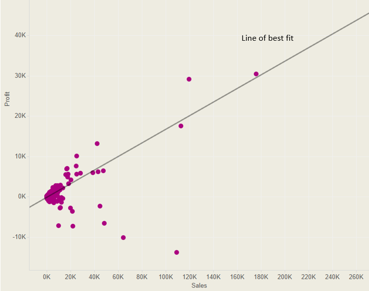
Linear regression is a way of demonstrating a relationship between a dependent variable (y) and one or more explanatory variables (x). For example, on a scatterplot, linear regression finds the best fitting straight line through the data points. It is used to identify causal relationships, forecasting trends and forecasting an effect. The line of best fit comprises analysing the correlation, and direction of the data; estimating the model; and evaluating the validity of the model.

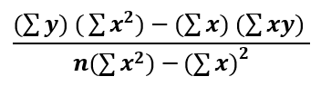
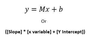
The regression line is calculated by finding the minimised sum of squared errors of prediction. In order to calculate a straight line, you need a linear equation i.e.:

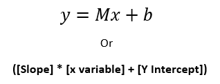
Where M= the slope of the line, b= the y-intercept and x and y are the variables. Therefore, to calculate linear regression in Tableau you first need to calculate the slope and y-intercept.

 

Calculating the Slope

In order to calculate the slope of the regression line you need to use this formula…but translated into Tableau:

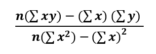
Where n = SIZE, x and y are the variables, and  = window_sum.

Once you break up this formula into 4 parts, it’s relatively easy to translate into Tableau. For this example, x = Sales and y = Profit.

Part 1: this is simply SIZE multiplied by the window_sum of x*y

(SIZE()*WINDOW_SUM(SUM([Sales])*SUM([Profit]))

 

Part 2: this is the window_sum of x * the window_sum of y

WINDOW_SUM(SUM([Sales]))*WINDOW_SUM(SUM([Profit])))

 

Part 3: this is SIZE multiplied by the window_sum of x²

(SIZE()*WINDOW_SUM(SUM([Sales])^2)

 

Part 4: the final part is (the window_sum of x)²

WINDOW_SUM(SUM([Sales]))^2)

Now you have the four components they need to be put together: (Part 1 – Part 2) / (Part 3 – Part 4) which looks like:

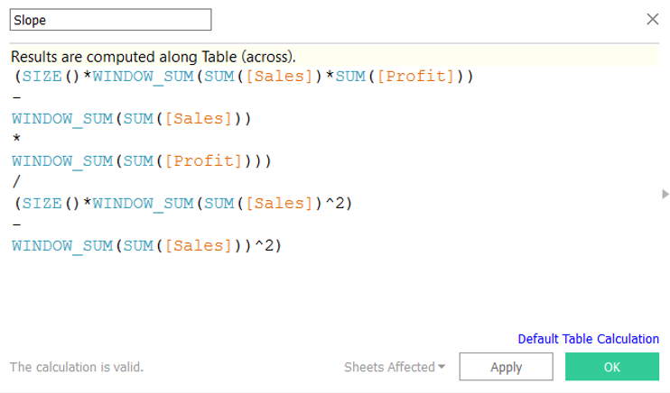
(SIZE()*WINDOW_SUM(SUM([Sales]) * SUM([Profit]))-WINDOW_SUM(SUM([Sales]))

*

WINDOW_SUM(SUM([Profit])))

/

(SIZE()*WINDOW_SUM(SUM([Sales])^2)

–

WINDOW_SUM(SUM([Sales]))^2)

 

Calculating the Y-Intercept

The y-intercept is where the straight line crosses the y-axis, and therefore the x value is 0. To work out the y-intercept you need the following equation:

Again, this can be broken down into four parts to make it easier to understand.

Part 1: this is simply the window_sum of y multiplied by the window_sum of x²

(WINDOW_SUM(SUM([Profit]))*WINDOW_SUM(SUM([Sales])^2)

 

Part 2: this is the window_sum of x multiplied by the window_sum of x*y

WINDOW_SUM(SUM([Sales]))*WINDOW_SUM(SUM([Sales])*SUM([Profit])))

 

Part 3: this is SIZE multiplied by the window_sum of x²

(SIZE()*WINDOW_SUM(SUM([Sales])^2)

 

Part 4: the final part is (the window_sum of x)²

WINDOW_SUM(SUM([Sales]))^2)

Now you have the four components they need to be put together: (Part 1 – Part 2) / (Part 3 – Part 4) which looks like:

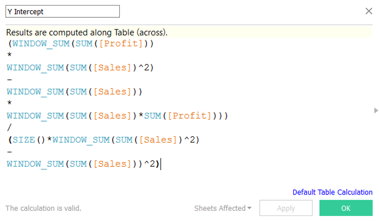
(WINDOW_SUM(SUM([Profit]))

*

WINDOW_SUM(SUM([Sales])^2)

–

WINDOW_SUM(SUM([Sales]))

*

WINDOW_SUM(SUM([Sales])*SUM([Profit])))

/

(SIZE()*WINDOW_SUM(SUM([Sales])^2)

–

WINDOW_SUM(SUM([Sales]))^2)

 

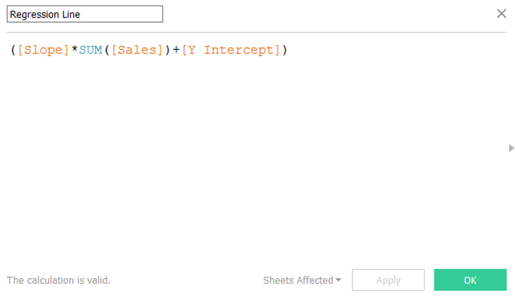
Calculating the Regression Line

Now that you have the slope and the y-intercept calculations you can use them to calculate the regression line:

 

Building a Visualisation

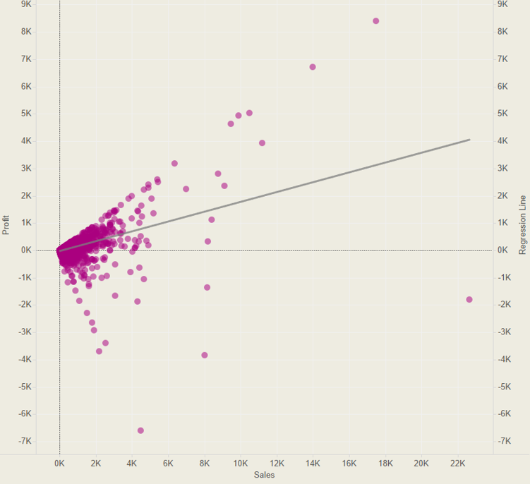
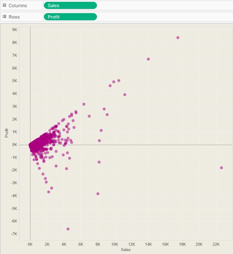
To use the regression line calculation in a viz, you can create a basic scatter plot by dragging Sales on to Columns and Profit on to Rows.

 

Then simply drag the Regression Line calculation on to Rows.

 

 

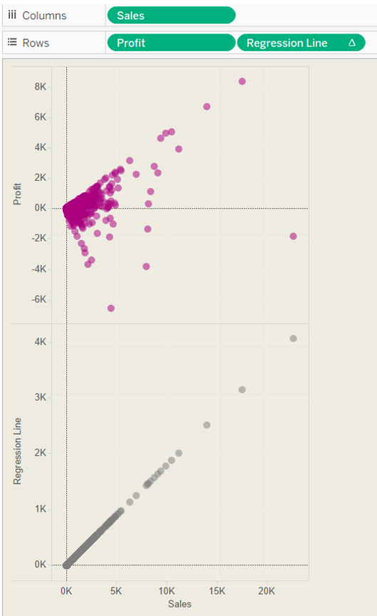
Now you can right click on the regression line chart y axis and make it a dual axis, synchronise it and your scatter plot and regression line are plotted on the same chart.

Next, you just need to change the regression line chart type to a line.