


Simply put, scaffolding refers to the process of adding rows to a dataset to achieve a higher level of granularity. This is useful for when we need to analyse data points that don’t explicitly exist in the original dataset.
This technique is most commonly used when working with dates, where certain time periods may be missing but still need to be represented for accurate analysis. Scaffolding fills in these gaps, giving you a dataset that behaves the way you’d expect for analysis.
Much like scaffolding in construction supports workers as they build, scaffolding in data supports analysis by providing the rows needed to work with a more complete and consistent dataset.
Let’s look at a simple example to put this concept into practice!
Let’s say you’re a gardener and you suspect you’ve been over-watering your plants, perhaps because you've accidentally been watering on days it’s already rained. To get a better understanding of this, for the next month you decide to track rainfall by writing down the date every time it rains. On dry days, you don’t record anything. At the end of the month, your data only contains rainy days.
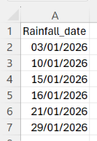
If you then want to see which days had no rain, and therefore how often you watered the plants, you would need a row for every day – which you currently don’t have. This is where scaffolding comes into play, let’s see how this can be done in Tableauprep using new rows.
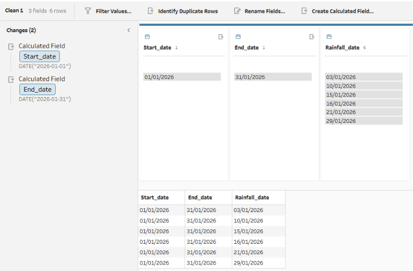
Before we get to that, we first need a clean step after loading in the data, where two calculated fields are created. 'Start_date' with the calculation DATE("2026-01-01"), and 'End_date' with the calculation DATE("2026-01-31"). We want a row for every day of January, so by ‘hard-coding’ the 1st and the 31st we define the boundaries of our calendar.
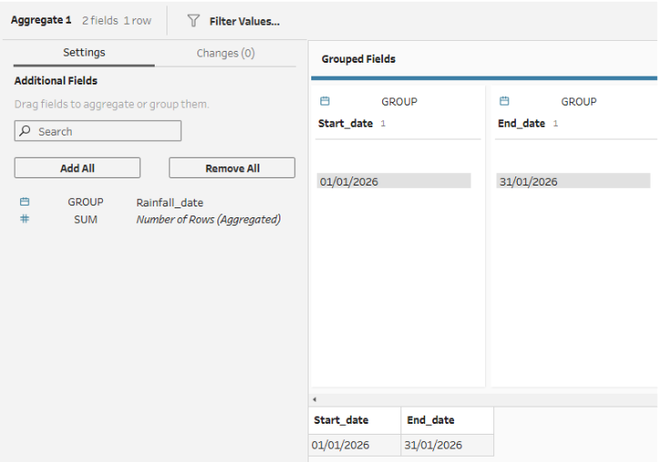
Because these new fields are added to every row of the original data, we need to use an aggregate step next, grouping by 'Start_date' and 'End_date'. This 'squashes' the data down to a single row so that when we generate the new dates, we don't accidentally multiply our rows.
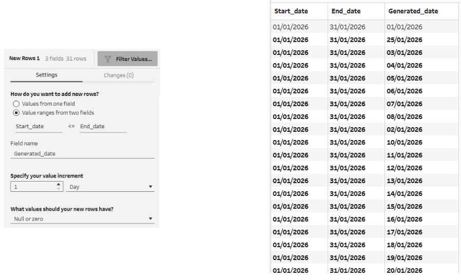
Now, we can use the new rows step, choosing to add new rows with value ranges from two fields and selecting these two fields to be 'Start_date' and 'End_date'. 31 rows will be created, as every day between the 1st and 31st inclusive is filled in.
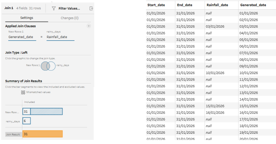
Now that we have a complete 31-day calendar, we need to bring back our original rainfall dates. This can be done using a join step connecting the new rows step with the original data. This will be a left join (keeping all the rows from the 31-day calendar side), with the join clause as Generated_date = Rainfall_date. This keeps the calendar intact, while matching up our generated days to the specific days it actually rained.
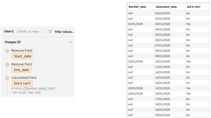
Finally, we’ll add one last clean step to interpret our results. First, the Start_date and End_date columns can be deleted, as they are no longer needed. Next, since the dates it didn't rain won't have a match from our original list, the Rainfall_date field will be null for those rows. We can use a simple calculation to label them in a new field called 'Did it rain?':
IF ISNULL([Rainfall_date])
THEN "No"
ELSE "Yes"
END
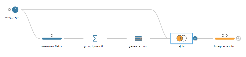
Ultimately, by filling in those gaps in the dates, we’ve turned a scattered list of rainy dates into a garden diary. We can now clearly see exactly which days it didn’t rain and how often we had to step in with the watering can. If you've been following along, your flow so far should look like this:
Of course, this is just a simple example, but in the world of data analytics, it’s important to remember that missing data is still data. Whether you’re tracking rainfall in your backyard or customer churn in a business, scaffolding can help you see the whole picture rather than just a collection of isolated data points.