


Hello! Come in and take a seat. Today, we're learning about how to aggregate in Tableau Prep, Power Query and Alteryx (the 3 data preparation platforms which we learn during training at The Data School). In case you weren't aware, this blog is actually part of a 'Back to Basics' series that I'm writing on fundamental steps in data preparation. I've covered about 5 or 6 topics so far and I'm always looking to cover more so head over to my profile if you're looking to level up your data preparation game and check out what I've written. Today though, let's explore aggregation!
What even is aggregation?
I feel like the word aggregation gets thrown around a lot in data preparation but the meaning can sometimes get a little lost in my brain at least - it's not like I use aggregation in day-to-day language unless I'm at work talking about data! A brief google says that the definition of aggregation from Oxford Languages is:
'The formation of things into a cluster'
I think this works quite neatly for aggregating in data preparation too because although I used to think aggregation was all about summing, it isn't always summing. You can aggregate with the AVG function, the MIN function, the COUNT function - the possibilities are endless really (actually they're really not because there are a set number of functions you can use but it's more than I can name right now!).
When you aggregate, you remove some of the granularity of the data which creates the aforementioned 'clusters', and means that you take it to a higher level of detail. Contrary to popular belief, a higher level of detail corresponds with a broader scope of data. I think a good way to consider this is through the term 'higher-ups' with a higher-up being someone who oversees parts or even the whole of an organisation. They're not the boots on the ground, working away at the minute details, they're looking at the bigger picture which is essentially what a higher level of detail offers - information about an overall grouping rather than a record on its own.
Today's Aggregation Functions
Today, we're going to go through a few different types of aggregation functions, both the typical ones that you'll use more regularly and ones that you might not be so familiar with but are good to know in case you need them.
SUM
This is the simplest of the aggregation functions that you'll probably be well aware of. This adds up all the numerical values within the group.
MINIMUM
This finds the smallest value within the group and returns it, when considering a numerical field. It also works for string fields to return the value earliest in the alphabet but I feel this is a less useful output. That's why it's important to ensure your numerical values are recorded as numeric data types, otherwise a value of 100 could be seen as the minimum over a value of 2, simply because the 1 in 100 comes before 2 in the lexicographical alphabet where strings are ordered on a unit by unit basis, rather than as a whole like numbers.
AVERAGE
This finds the mean numerical value of the group using the sum of the group values divided by the number of items in the group. It is important to consider how nulls are treated by each platform as this will impact the result that is output. This is something we'll review, specific to the software.
COUNT
Count is typically used with string values to determine how many occurrences of something there is, but it can be used with numerical values too. There is also a COUNTD (count distinct) option too which only counts the unique values in the column (e.g. in the superstore dataset, as rows are at the product level within an order, the order ID doesn't get recounted if using COUNTD).
STANDARD DEVIATION
Standard deviation is our first measure that's a little more intense on the statistical side of things. It explores how closely the data points are spread around the mean with a low standard deviation indicating a more closely clustered dataset.
PERCENTILE
Writing this blog post, I too discovered what the percentile function was which is likely indicative of how often I've used it (i.e. not at all so far). The percentile function returns the data value in the specified percentile of the dataset. For example, the 50th percentile value returns the value located in the middle of the dataset if the values were in ascending order. This is actually the median. A high percentile value will return a value closer to the upper limit of the dataset and conversely for a low percentile value.
Now that we understand the functions we're going to be exploring, let's dive into the platforms.
Tableau Prep
To aggregate in Tableau Prep, you require an aggregation step. This can simply be added onto the end of your workflow.
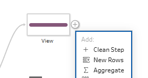
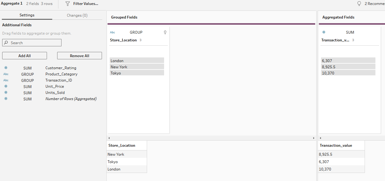
To begin with an easy one, we're going to find the total transaction value of each store location. This uses the SUM function. Simply add your aggregation step to the workflow, and set it up with your store location in the grouped fields section and your transaction value in the aggregated fields section.
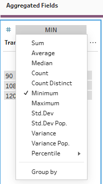
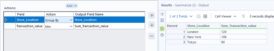
To find the minimum transaction value by store location, you can do exactly the same steps before changing the aggregation type from sum to minimum.
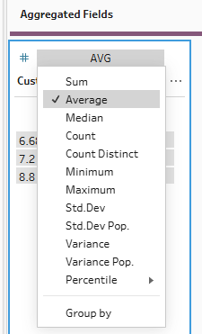
For the average function, we want to find the average customer rating by category. To do this, we change our group by field to category from location and we change the type of aggregation of our customer rating field to average.
How does this factor in nulls though? Let's look at the outputs if I keep the nulls in vs when I change the null to a zero.
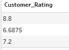
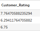
As you can see, null rows are naturally eliminated from the calculation. This is something to be careful to consider depending on what you're trying to show. If you're calculating customer rating, you wouldn't want the nulls to be included as zeros because this would drag the average down for no particular reason. However, if you were looking at average customer spend and a customer hadn't spent anything, it might be important for nulls not to be eliminated as otherwise you'll be leaving out a whole demographic of customers in your analysis.
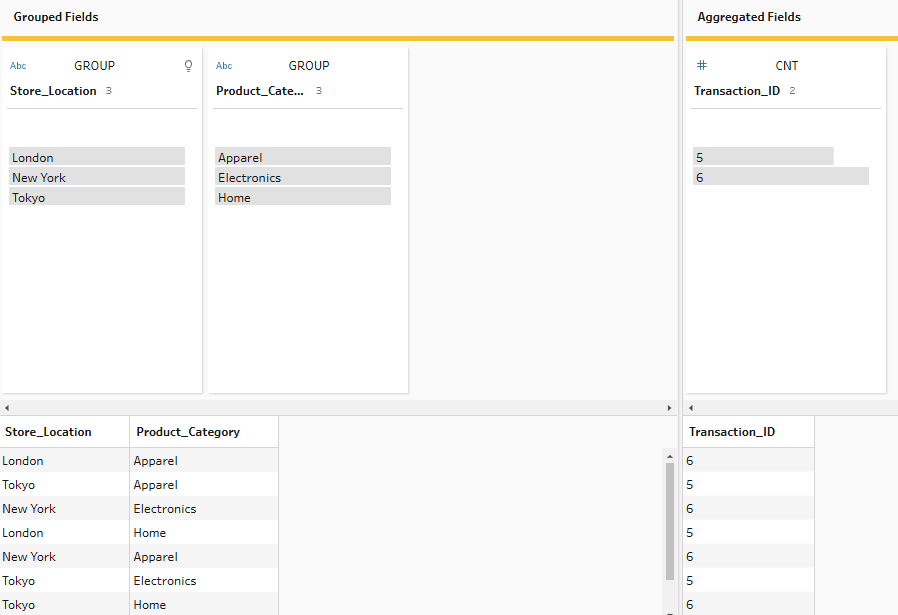
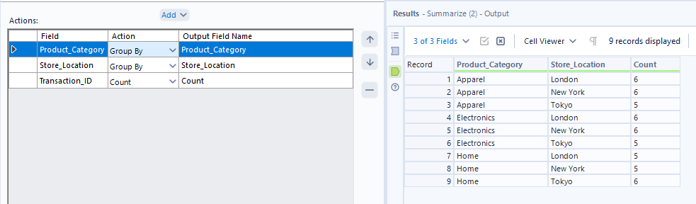
For the next aggregation, let's suppose we want to see how many transactions are taking place across each location x category combination. For this, we add both our location and category fields to the grouped fields side. Then we need to drag our transaction ID to aggregated fields and change the aggregation to COUNT. As we know transaction ID is unique per row, we can use COUNT rather than COUNTD as they will return the same output.
Now, into the more heavy duty statistical aggregations. Let's begin by looking at standard deviation of customer rating across product category. Simply follow the same steps as we have previously - adding product category to group and customer rating to aggregated fields. Then change your aggregation to standard deviation. The values are fairly low and as the overall values can only vary between 1 and 10, this makes sense.
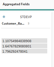
You might have noticed there is also a standard deviation population option. This takes into account the whole dataset whilst standard deviation takes into account a sample of the dataset. As our overall dataset is only 200 rows, and the values have a limited amount they can vary by anyway, the distinction between the two types of aggregation is minimal in this instance. But if you had a larger dataset, you might want to weigh up the benefits of the reduced bias for standard deviation population against the drawbacks of the increased processing power required.
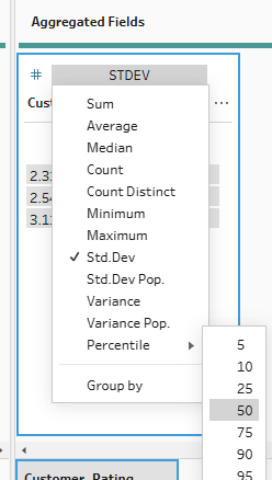
Our last function to explore in Tableau Prep is, of course, percentile. Simply use the same steps as above but change your aggregation type to percentile, specifying which percentile you'd like to return. I like 50 because it indicates the median average.
So, that's some of the key aggregation functions that can be explored in Tableau Prep - quite simple once you add your aggregation step in. My final key tip is that if you ever accidentally add the wrong field, you can just click on 'GROUP' or the type of aggregation and drag the field back to the settings pane to remove it. You don't need to delete the step entirely and restart. Anyway, let's see if we can step it up a level!
Alteryx
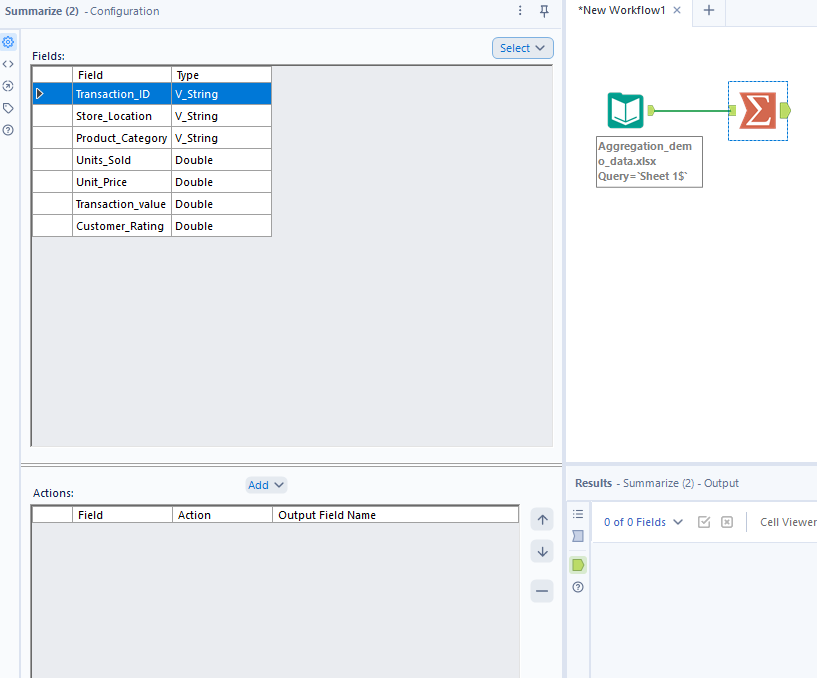
To aggregate in Alteryx, you follow fairly similar steps to those in Tableau Prep - the set-up just looks slightly different. Start by loading your data in before adding a summarise tool to your workflow. A configuration pane will pop-up on the left which is where you will specify how you would like to aggregate.
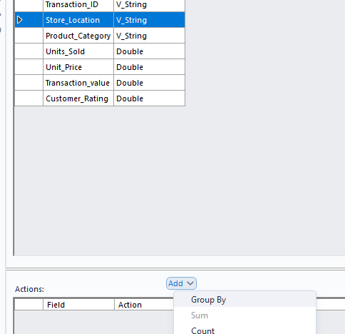
As before, let's start by finding the total transaction value for each store location. Click on store location, then click on add > group by. You might notice that certain options in the add section are greyed out (like sum). This is because store location is a string field and you can't perform the greyed out functions on certain data types.
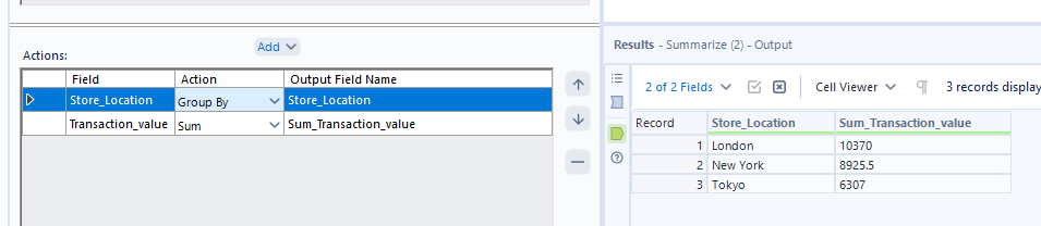
Add your transaction value with the 'sum' action and there you have your first Alteryx aggregation.
Again, to find the minimum transaction value by store, simply change the 'action' from sum to minimum.
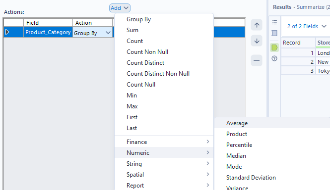
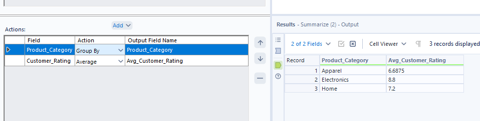
Next, let's look at average customer rating by category and see how nulls are incorporated in Alteryx. You might notice that when you try to find customer rating in the regular add dropdown, the option doesn't immediately appear. To find it, you have to go down to numeric, then find average.
Let's see how the averages compare when I convert nulls to zero in a formula tool before the aggregation.
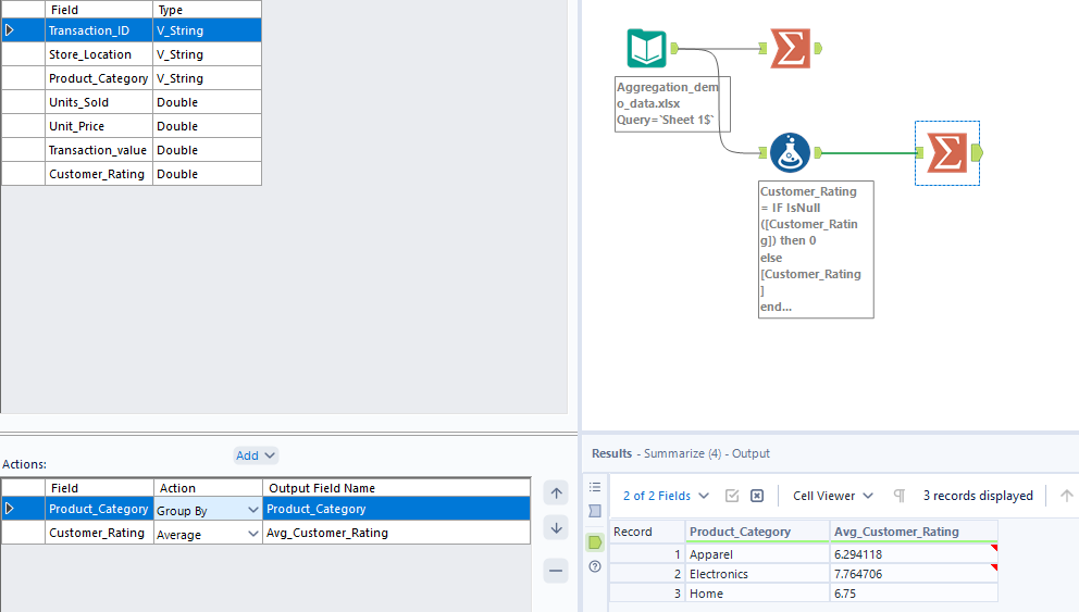
Again, we see the same situation as Tableau Prep so remember to consider your options carefully when averaging with nulls in Alteryx!
Moving on to counting string values, simply add your extra group by field (store location) to the action pane and add transaction ID with the action 'count'.
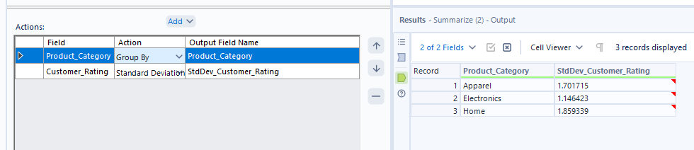
On the more significantly statistical side of things, we can add standard deviation to our arsenal by following the same steps as we did for average. In the add dropdown, go to numeric > standard deviation. Unlike in Tableau Prep, there's no differentiation between types of standard deviation and from my googling, it seems that the default and only option is using a sample population. You do have a different option though to exclude zeros from the calculation if you so choose. In this instance, I don't have any zeros anyway so we get the same output either way.
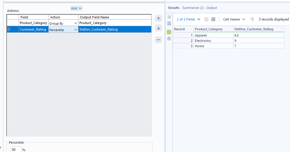
For percentile, you can follow the same steps as above but opt for percentile in the numeric options instead. You can choose what percentile value you'd like to return by typing in a number between 0 and 100 into the box at the bottom of the action pane.
And that's a broad summary of aggregating in Alteryx complete. If you ever add the wrong category by accident, remember you can remove it by selecting the category (making it highlight in blue like customer rating above) and clicking the minus button. Now let's look into our final platform!
Power Query
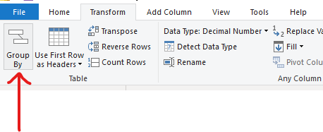
As I'm sure you're already aware, the Power Query set-up looks quite different to Alteryx and Tableau Prep but the fundamentals remain the same. After loading the data in, we'll start with a simple summing of the transaction values per store location. To do this, go to the Transform tab and click group by.
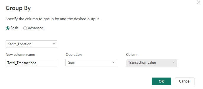
Then set up your pop-up window so that you're grouping by store location, naming your new column however sensibly you please (I'd suggest Total_Transactions but to each their own), adding your operation as sum and your column as transaction value.
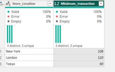
To get the minimum transaction value, do the same steps but use the minimum operation instead.
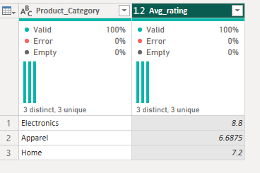
Again, let's turn to the slightly more complicated world of averages by altering the grouping column to category and the column being aggregated to customer rating, as well as the operation type to average. As with the other platforms, the nulls are excluded from the calculation - just something to note for today.
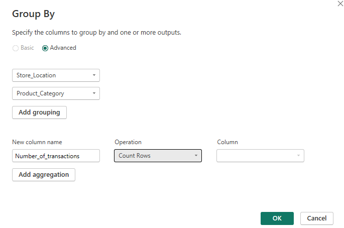
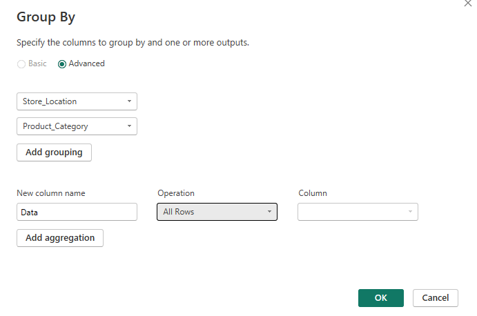
For the count function, we have a couple of fun new things to learn. As we wanted to count the number of transactions by location and category, we need two group by categories. However, in the basic option, we can't do that so we move into the advanced pane. Very fancy. We fill that out as appropriate and then you might notice that there's no specific count option. We can count rows but we can't specify which columns to count by.
For today's option, that works. I know that there are no repeated transaction IDs so the number of rows returned will be the number of transactions. But what would I do if I had a sample superstore dataset and I wanted the number of orders? There's an option to count distinct rows but that's not going to fix the issue because the rows themselves are unique, it's only the order ID specifically that isn't. So how do I work this out?
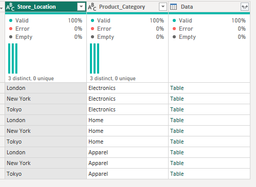
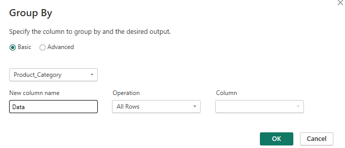
To fix this, you essentially need to create a grouped table initially, setting up the aggregation in the same way but using 'All rows' as the operation.
You then need to create a custom column to count the distinct transaction IDs. If you read my rank blog, this will likely be feeling a little familiar!
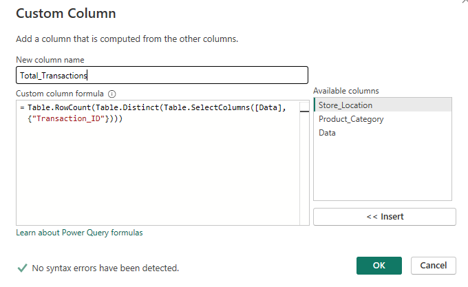
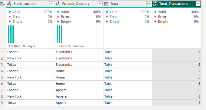
Working from the outside in, the calculation is asking for the transaction ID column from the Data table that we just formed. It wants the distinct rows in this table (as we're only returning transaction ID, it's only looking at the distinct values within transaction ID) and then wants to count the number of rows there are. It does this for each mini table per location x category grouping.
That was a little heftier than expected! However, it is going to make our lives a little easier when understanding how to calculate standard deviations and percentiles as neither of these options are found in the group by pop-up window.
We're looking at customer rating by category and the statistical analysis for this combination. Let's start by creating that same table we did before by going to group by category, operation 'All Rows'. We then need to create our new custom columns.
Starting with the standard deviation custom column:
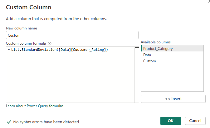
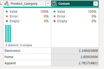
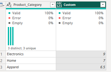
To translate, this calculation is saying write the standard deviation for the customer rating column within the 'Data' mini tables (a mini table is at the category level). I should name things more excitingly to make it more obvious but this name is based off the column name that we used in the initial group by step. Of note, like in Alteryx, standard deviation is calculated on a sample population and there is no option to calculate the standard deviation of the overall population.
For the percentile custom column, follow the same initial grouping steps but copy out this calculation instead:
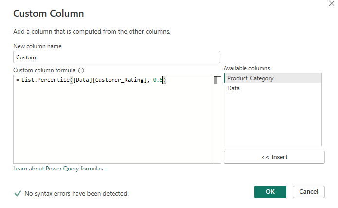
Similar to the translation above, this calculation is expecting to output the 50th percentile of the customer rating value in each 'Data' mini table (with a mini table per category). You can change the percentile value you wish to output by editing the '0.5' at the end of the calculation to any number between 0 and 1.
So that's how you aggregate in three key data preparation platforms: Tableau Prep, Alteryx and Power Query. It did get a little less straightforward at the end there so well done for keeping at it. We made it through and now have another chunk of knowledge to add to our bank!
I think the final thing to note which I surprisingly haven't done so already is that you don't need to use group if you don't want to. You might want to find the overall average transaction value, for example. I expect you typically will want to use group by because otherwise you're just outputting a single value which isn't much use during data preparation though. But if you wanted to find the average transaction for example, then cross join or append that single value onto the original table for comparison, you could. The way that you can aggregate without a group by field is quite simple honestly, just don't add a group by field. This is a little different in Power Query as you have to go to advanced and then click the dots to delete the pre-entered group but it's still possible. Anyway, that's my final nugget of wisdom for the day. Until next time, happy prepping!