


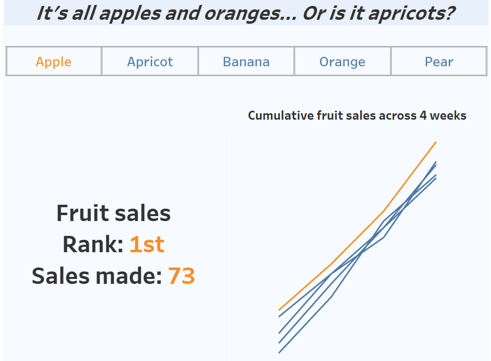
I'll begin by admitting that this is a rather niche blog post but during my application to the Data School this was exactly the post that I could have used. I had a vision and nothing was going to get in my way of achieving it, even if it took far longer than it probably should have to get there. There were a few stumbling blocks along the way which I'll take you through step-by-step but by the end, you'll have a functioning dashboard which you can add to and make your own. So, if you have ever wondered/struggled with how to create a category toolbar (see the image below for what I mean by this) and how to use it to filter ranked values, this blog post is for you. And even if you haven't, this post can be for you and your future ranking dashboards too.

Creating a Category Toolbar
This is an incredibly simple but effective addition to any dashboard to highlight or filter other worksheets. It's more visually appealing than a regular drop down menu and I think it looks like you've gone that extra mile whilst only having to do maybe a few hundred yards worth of effort - I've lost myself in imperial units now but the extra kilometer just didn't have the same ring to it.
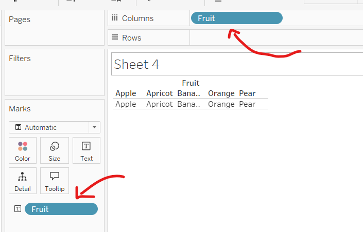
Step 1: Add your category to the columns and the text box on the marks card.
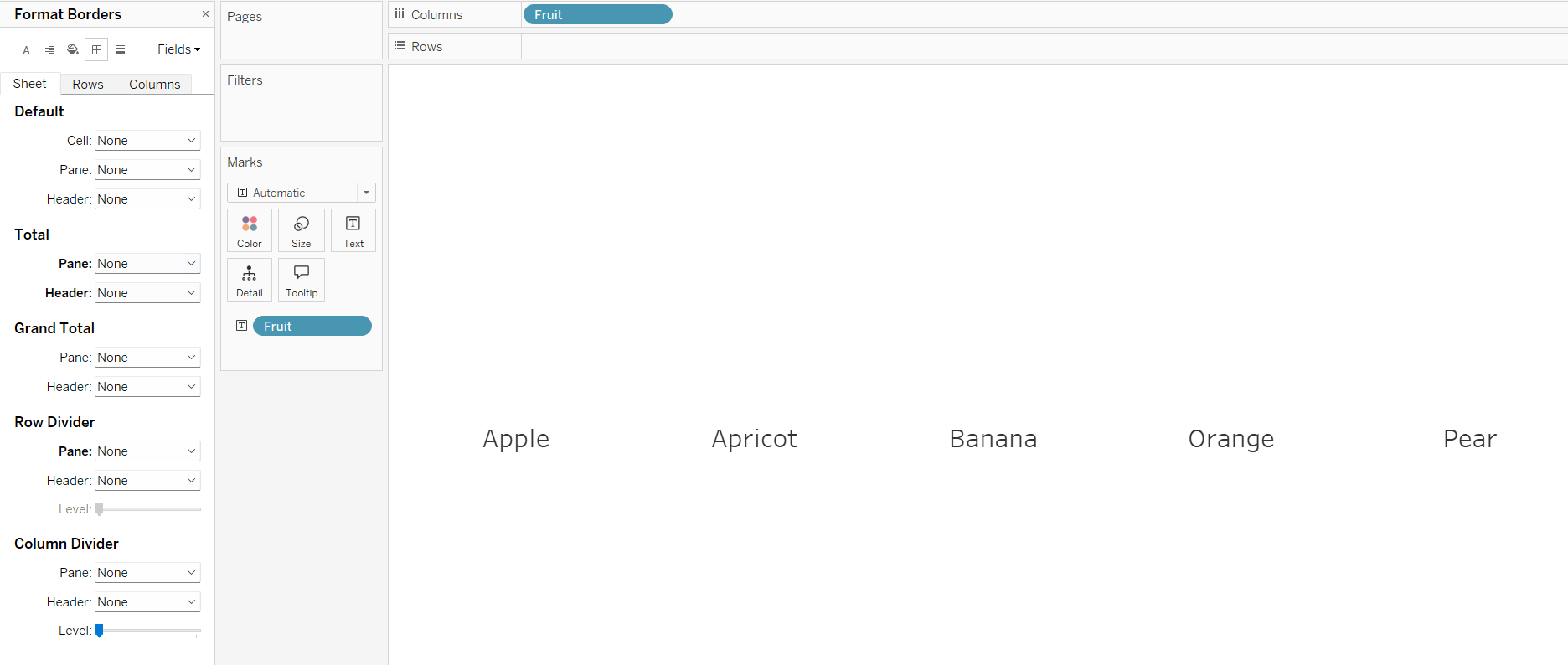
Step 2: Clean it all up by hiding the header, adjusting the row divider in the pane and cell border, increasing the size of the text and aligning the text to center in the pane. N.B. The screenshot below doesn't have the bordering yet.
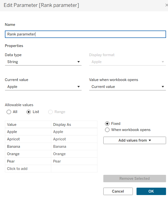
Step 3: Create your category parameter by changing the data type to a string and changing the allowable values to a list, individually adding each of your categories (in this example: apples, oranges etc.). Ensure that when the workbook opens, it opens at the current value and typically that will be the top value in your list.
So, now the basic framework has been set for the category toolbar. There will be a few extra steps needed for it to interact with your ranking worksheet but first, onto creating that.
Creating your rank card
Step 1: To create a rank card. you first need to create a table calculation to get your individual ranks. This is very simple and all you need to do is use the rank function on whatever measure you're ranking by. I used the following calculation:
RANK(SUM([Sales]))
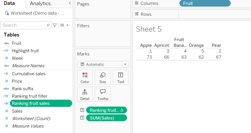
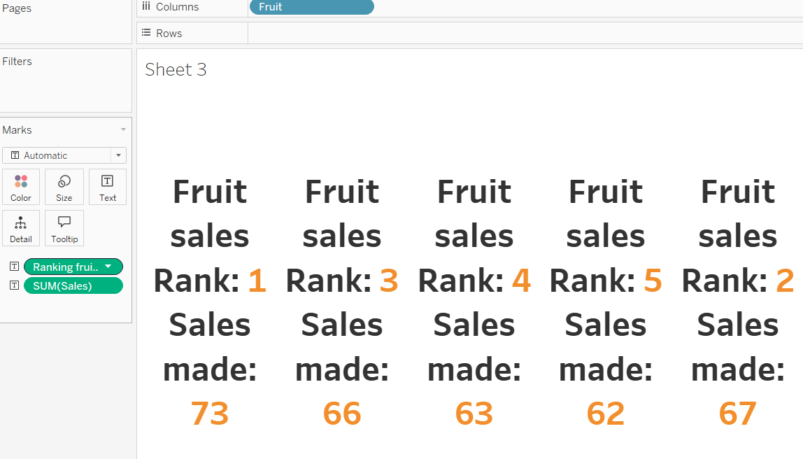
Step 2: Drag category to columns and add your rank calculation to the text box on the marks card. You can also add any other fields that you'd like to be on your marks card to the text box now. For example, I wanted the cumulative sales of my fruit to add context to my ranking.
Step 3: Clean it up. Get rid of the header and reformat the text as you wish to do so by selecting the text box in the marks card and clicking the three dots that appear. Personally, I also like to remove the row divider in the pane but do what you think would suit your dashboard best.
Step 4: This is an optional step that really depends on what you're using your ranking for and what you want to show based on personal preference. For me, in my original application my rank represented final outcome in a championship so it made more sense to me to say they finished in 1st, 2nd, 3rd position etc. However, I probably wouldn't normally do it for fruit sales because that's not typical terminology used. Still, I've added the ordinal suffix in this instance to help you if that's what you're looking for and save you an extra google search! Copy out the code below with your ranking field inserted.
IF (RIGHT(STR([Ranking fruit sales]),1)= '1') THEN 'st'
ELSEIF (RIGHT(STR([Ranking fruit sales]),1)= '2') THEN 'nd'
ELSEIF (RIGHT(STR([Ranking fruit sales]),1)= '3') THEN 'rd'
ELSE 'th'
END
If you're interested in what the calculation means, it is converting your rank value into a string so it can compare your number and your suffix. The right bit is saying the positions from the right that you are using and for our case doesn't make a difference, but would do if you had double or triple digit numbers as it would only take the end digit. Because of the nature of the category toolbar, you shouldn't be going above 10 categories I expect but if you were planning to, you will need to add extra clauses as, for example, both 1 and 11 end in 1 but they have different suffixes.
Filtering your rank card
Now we're getting to the good bit! You need to put your dashboard together now - don't worry that you haven't filtered the rank card yet because we're coming to it. I added an extra worksheet to highlight how sales accumulated over the four weeks for each fruit and if you have other worksheets, you might want to do something similar. As I am using a filter (where all values are excluded except from the one associated with my selected category) for the rank card but a highlighter (where all values get greyed out but are still visible and the selected category is coloured to stand out) for the other worksheet, I do need a separate parameter action. If you want to add to your dashboard with highlight actions, you can follow a step by step from this blog post which was my original inspiration: https://www.thedataschool.co.uk/a/eve-thomas/creating-a-simple-highlight-parameter-action-in-tableau. If not, carry on to filtering your rank card or you can come back to this afterwards. It isn't order specific!
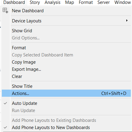
Step 1: Remember way back when we created a category parameter all that way up the page? Well this is its starring moment. In your dashboard, go to dashboard in the toolbar at the top of the screen followed by actions. Then click add action and change parameter.
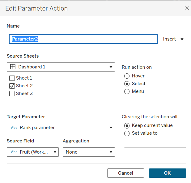
Step 2: In this edit parameter window, ensure that your dashboard is the source location with the source sheet being your category toolbar (name your worksheets unlike what I've done here!). Your target parameter is your rank parameter and the source field should be your category. Ensure that you are running the action on select (unless you want to do hover but just take into account what you've chosen) and clearing the selection will keep the current value. The second bit is very important because otherwise things will get very confusing!
Step 3: Nothing will have happened yet. That's okay. You need to do one final thing to get it all working smoothly. Go back to your original worksheet with your rank cards and create a calculated field. Now, the key step here is to realise that if you just used a regular filter, every time your parameter action filtered your rank cards to just show one card, it would claim that each of your fruits was ranked 1st. That's because of the order of operations that Tableau follows (think BIDMAS but for Tableau) where it ranks after the filter has taken place. Therefore, you have to use the following calculation to find the rank for the overall fruit sales:
LOOKUP(Max([Fruit]),0) = [Rank parameter]
Step 4: The last thing you need to do is add your calculated field to the filters card and select true to show only your selected fruit category.
And there you have it. Hopefully this has helped you solve a question that you had about category toolbars or filtering rank cards, or given you some fun ideas to include in a future project. For now, onwards to week 4!