


Today DS12 had their first stats 101 class, an introduction to statistics which covered the basics of normal distributions, standard deviations and p-values. One of the charts we learnt to make was a control chart, a chart used to show whether the variance in a measurement is within acceptable bounds, in this case, the standard deviation, which can be controlled by the user via a parameter. The chart can be seen below and this blog will aim to walk you through the creation process.
Creating the basic chart:
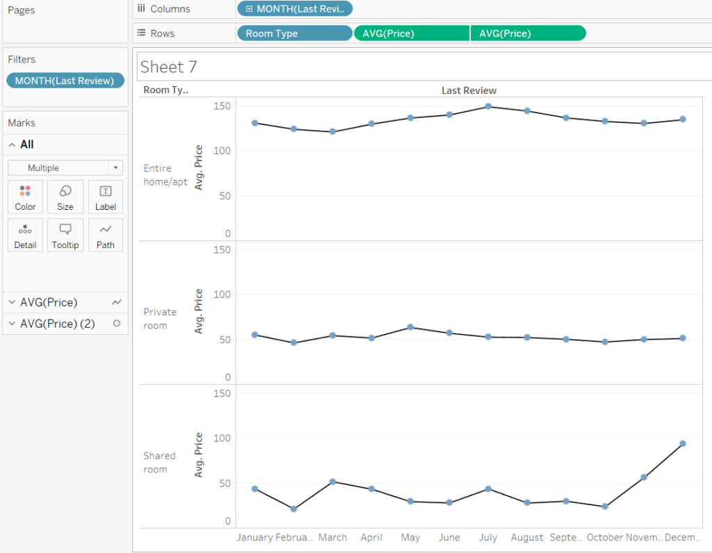
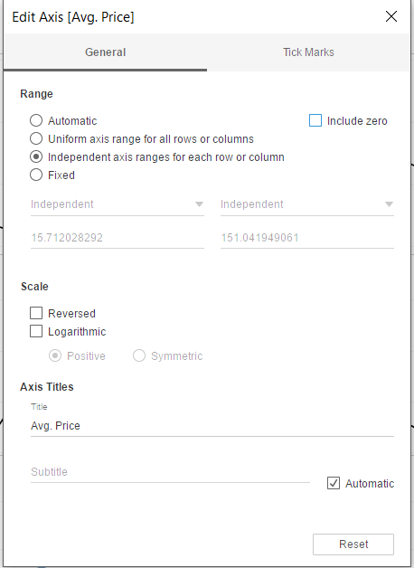
The data is from AirBnb, showing the how the average price of rooms varies throughout the months of the year. The data is also split into three panes, for the three different room types available. The first step is to build the basic underlying chart, without any parameters or distribution bands. I have put the month of the last review on the columns with room type and average price on the rows shelf. The average price has been duplicated and put on a dual axis, this is how you achieve the effect of having circle marks on a line chart (play around with line and circle colours and sizes as you please). I have also edited the average price axis so that there is an independent axis for each room type and that zero is not included (see picture below).
Creating the standard deviation parameter:
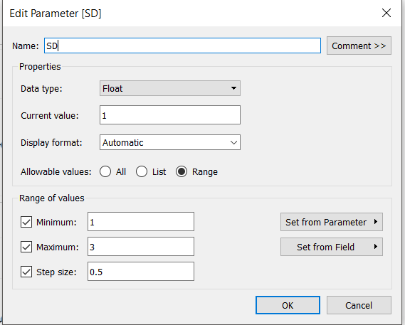
To create a parameter, right click on the white space in the measures/dimensions pane and select create parameter. You can see how I set mine up below. I used a range of 1-3, as it is highly unlikely that there will be data points outside 3 standard deviations. I also used a step size of 0.5, you must ensure your parameter is set to a float value in order for this to work. Once you’re set, show the parameter control on your sheet. At this point, it will have no effect on the chart, as we are yet to add our calculated reference bands.
Creating the necessary window calculations:
The next stage is to use create some window calculations for the average line and the reference line. The reason window calculations are used is because they calculate values across the whole pane, if I were to just use a normal calculation, it would calculate averages and upper/lower bounds for each individual data point. These are the three calculated fields I have used.
Average line: WINDOW_AVG(AVG([Price]))
Upper bound: [Window Average Price] + ([SD]*(WINDOW_STDEV(AVG([Price]))))
Lower bound: [Window Average Price] – ([SD]*(WINDOW_STDEV(AVG([Price]))))
Once you have created these, add them to your details shelf.
Adding calculations to average lines and reference bands:
First, drag a reference line from your analytics tab to the sheet, and set it to calculate for the pane. In the settings, use your average price calculation as the value. Remove any labels for a cleaner look. Next, drag on a reference band, again for your pane. In the settings for the band, add your lower bound calc to ‘band from’ and your upper bound calc to your ‘band to’. Again, remove the labels and edit the colours and lines to your preference. You will notice that you are now able to change the reference bands using the standard deviation parameter.
Adding colour for outliers:
The final step is to write a calculation that will colour marks one colour if they fall within your set standard deviation (normal) and another colour if they fall outside this (outlier). This is the calculation that I used, however, it could also be written in other ways, such as a true/false statement.
IF AVG([Price (copy)]) > [Upper Bound ] OR AVG([Price (copy)]) < [Lower Bound] THEN “Outlier”
ELSE “Normal”
END
The calculation simply states, if a value is greater than the upper bound, or greater than the lower bound then it is an outlier. This will allow the colours of the marks to change as you change the standard deviation and marks may change from normal to outliers. Add this to colour on your circle mark types, and you should have a fully functioning control chart!