


Tableau's dynamic updating and interactivity is among its best features, but they can be limited when trying to perform statistical analyses. These kinds of analyses rely on many sequential calculations, often end with references to statistical distributions that are beyond the scope of Tableau's mathematical capabilities. In this blog, I will describe how I used RServe integration in Tableau alongside LODs (level of detail expressions) to develop dynamic Chi-Squared testing for Tableau!
What is a Chi-Squared Test?
The most well known statistical procedures involve 1 or more quantitative variables. To evaluate a difference in means or proportions across two categorical groups, analysts often use a z-test or a t-test. These kinds of tests are performed on slopes when checking if two quantitative variables are associated with each other. One way to check whether 2 categorical variables (dimensions, in tableau) are associated is using a Chi-Squared test. The idea behind the test is based on the null hypothesis that the two dimensions are not associated. If this was the case, then the table would be extremely uniform. Mathematically, the null hypothesis table has cells of the form:
Since the latter part of this blog consists of an application to the Tableau default Sample - Superstore dataset, I will phrase most of my examples in that language. The question of interest for this analysis: is there an association between Region and Segment? The counts for this analysis are numbers of order IDs associated with each of the combinations.
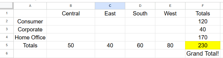
As an example, we would compute the expected value for the Consumer segment in the Central region as 50 * 120 / 230 = 26. The result of this formulation is that every cell will be proportionally represented based on the totals in its column, and in its row. In practice though, data is messy and things don't perfectly divide out like this. Maybe this cell is actually filled with 31 order IDs. Is that very different? This is where statistical testing comes in! Using this formula:
that finds a weighted sum of how far off each cell from the table is from the expected value, weighted by the size of the expected count. The last step of the test is to plot the newfound Chi-Squared statistic on a Chi-Squared distribution to find a p-value, the odds that a result as extreme or more extreme than the one observed could have appeared by random chance if our null hypothesis was true. This is where we will reach the boundary of native Tableau functionality and move to R, but there will be other interesting LOD challenges along the way. Let's get implementing!
Calculations
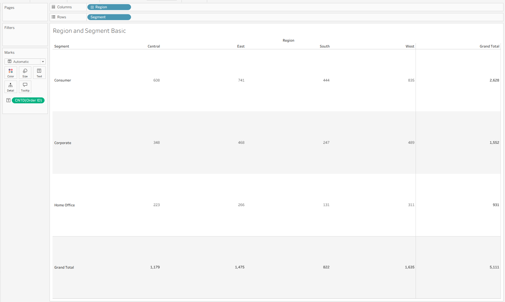
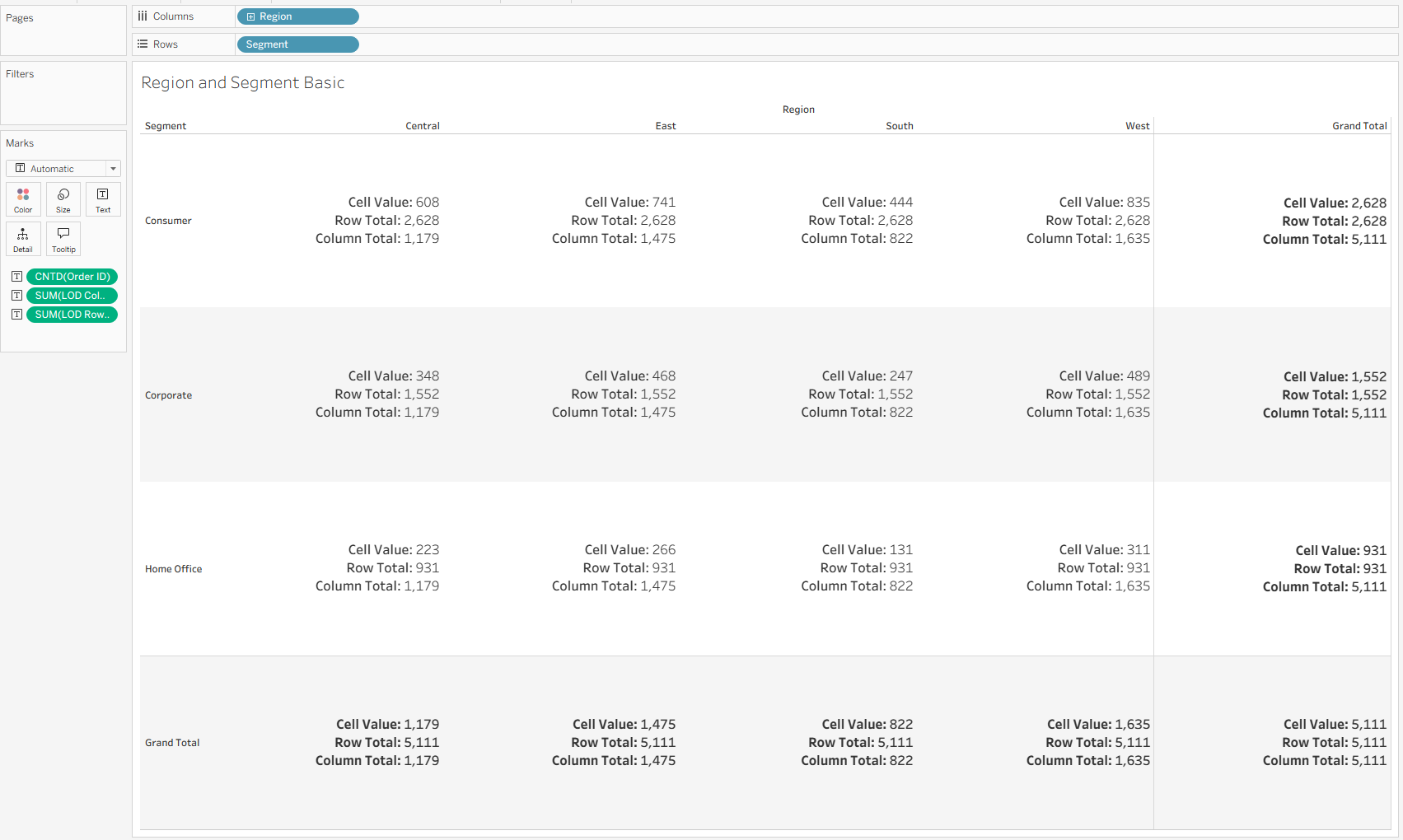
The first few steps in Tableau are not so calculation intensive – I dragged in Region onto Columns, Segment onto Rows, a distinct count of Order ID onto text, and added row/column totals from the analytics pane.
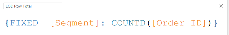
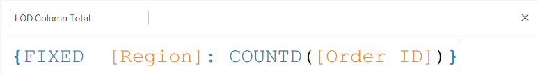
For the row and column totals, I used Level of Detail expressions, which fix on the corresponding variable to deliver the total counts across the row/column instead of at the individual cell level.
Now with a quick sanity check, we can see our table looks like this:
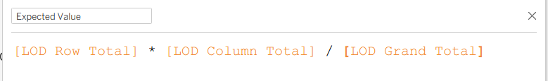
Next, we need to find our expected values, which we can compute using the following calculation, which uses the first equation included in this blog!
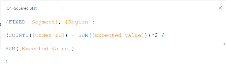
After this, we need the Chi-Squared contributions for each cell so we can later sum them to be the actual Chi-Squared statistic. To do so, I fixed on the fields that represented the rows and columns, and mirrored the Chi-Squared expression from above.
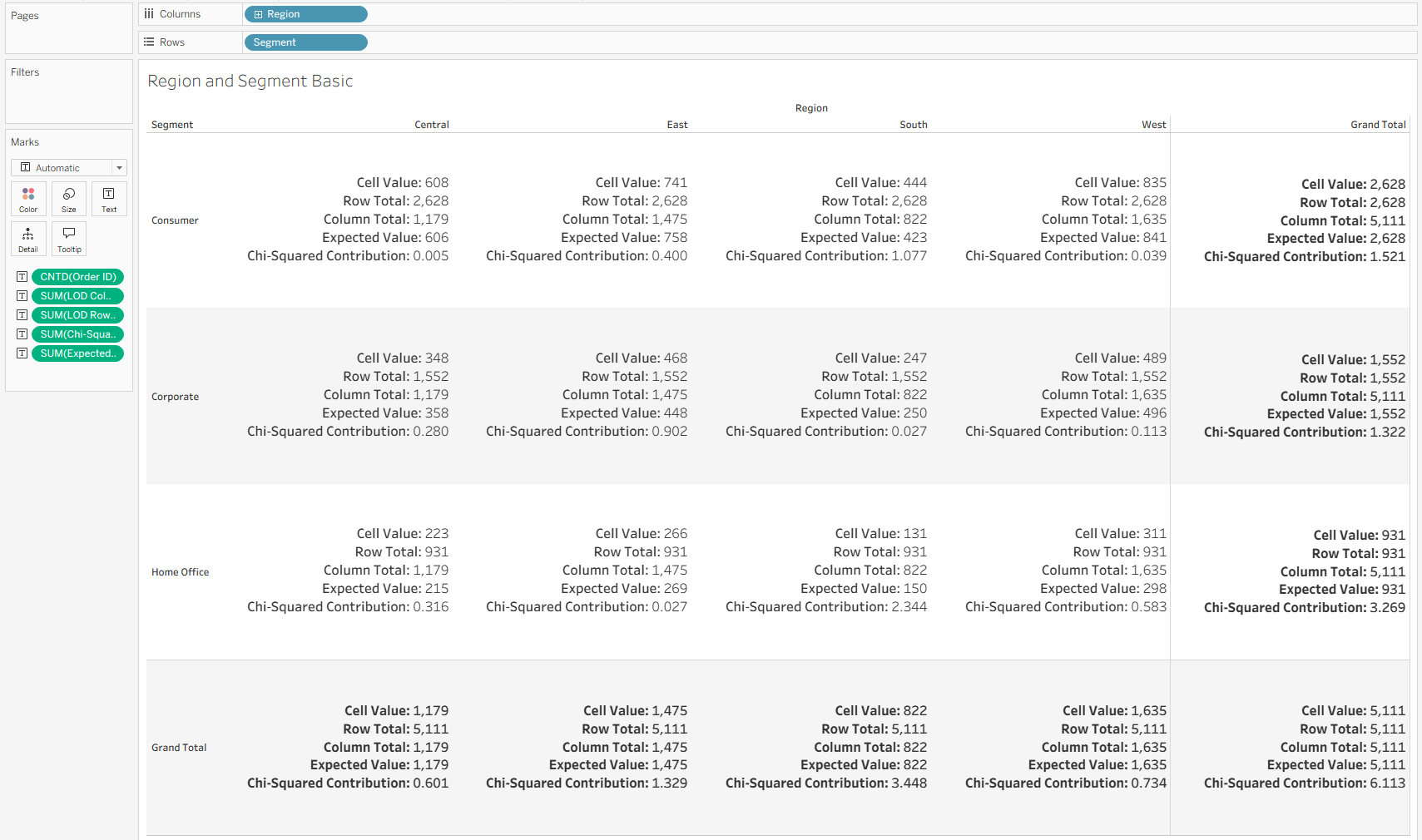
Here is the final "sanity check" table for the calculation building process:
It is definitely important to note that although I chose to implement this using Level of Detail logic, it can similarly be done using window functions (or the same window function:
WINDOW_SUM(COUNTD([Order ID]))
computed in various different ways (table down, table across, etc.). I chose to use LODs in this case to make sure things were not so dependent on the view, so that I could check my summations in a different sheet:
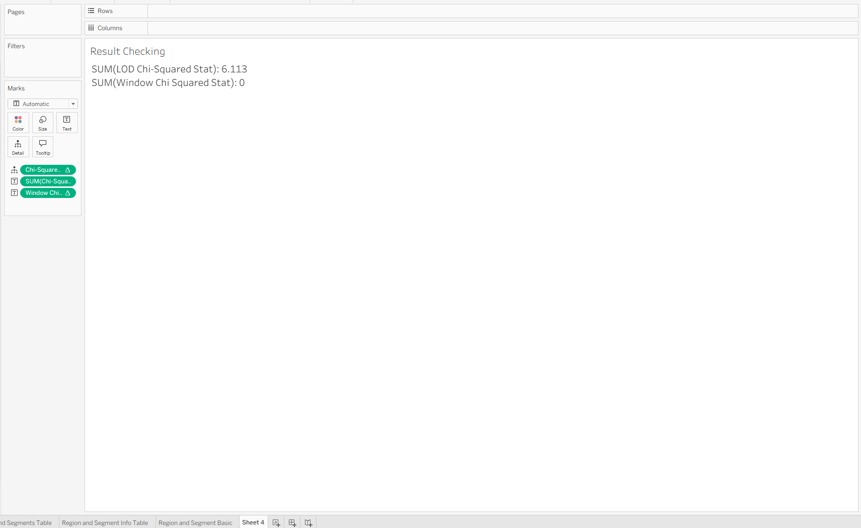
Since the window functions are dependent on the view, this new sheet does not carry through the logic, although within one sheet, they work the same. In fact, the window functions are more flexible than the LOD logic because of where they sit in the order of operations (last!). Getting the LOD logic to be dynamic will require more resourceful uses of context/data source filters, but is still possible.
These caveats should not distract from the excitement that this worked! We now have a Chi-Squared stat that sums the contributions from all the cells. The last step is to see where 6.113 lies on a Chi-Squared distribution.
R Integration
For a more in-depth explanation on how to integrate R into Tableau, I will refer you to Le Luu's two part data school blog series (Part 1, Part 2).
The most important part of the story on the Tableau end included navigating to the analytics extension page using the help menu,
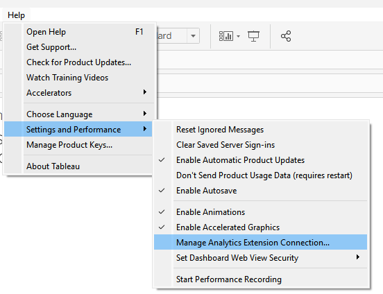
and selecting RServe once there:
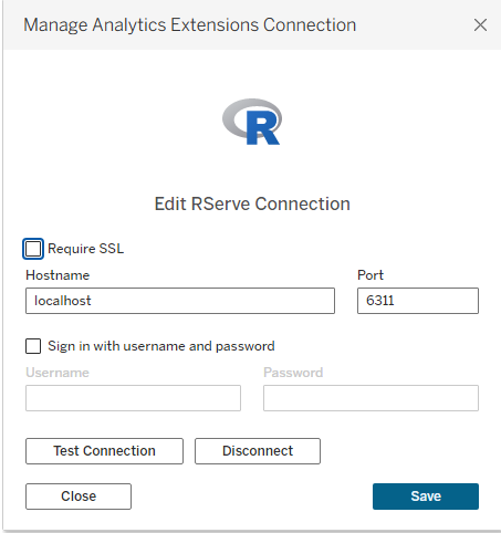
I will leave the other details to Le and Tableau's documentation, but the connection worked pretty seamlessly!
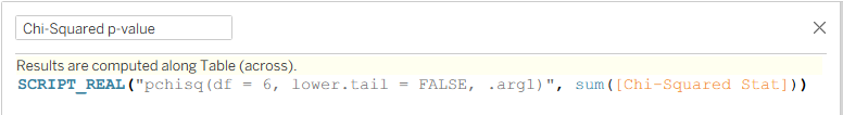
To write R in Tableau, users can use the functions SCRIPT_REAL, SCRIPT_BOOL, SCRIPT_INT, and SCRIPT_STR within normal calculated fields. These arguments take R syntax as a string as their first argument, and a list of Tableau fields/calculations after that to feed into R.
In my case, I used the SCRIPT_REAL function, which returns floats, and used the pchisq function based on this R documentation to find where 6.113 lies on the corresponding distribution. In this case, "df = 6" means the distribution has 6 degrees of freedom. This can be calculated by multiplying the row count - 1 by the column count - 1, so in this case (4 - 1) * (3 - 1) = 3 * 2 = 6. Last, I used the ".arg1" syntax to reference the Tableau calculation that came next, which is the same calculation used to find that 6.113 figure shown above!
After adding this calculation to text, Tableau takes a second to call R to do the calculations and comes back with this:
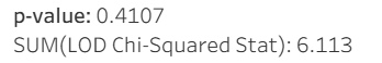
A p-value of 0.4107 means that if our null hypothesis was this extreme, the chances of us seeing a Chi-Squared stat of 6.113 or higher would be about 41%, which by typical statistical standards is not that remarkable. There are many other great resources about how to interpret p-values, but this one is pretty clearly non-significant, meaning that we can conclude that in the Sample - Superstore dataset, there is no discernible association between Region and Segment.
For me, the most exciting part of this build is that it is dynamic. As a statistics student, I had to do this process by hand every time, but with this flow built into Tableau desktop, it can now dynamically return a new Chi-Squared statistic and p-value every time the data source is updated, and can even respond to filtering in real-time, assuming they are context filters (see Tableau's Order of Operations).
Integration with R opens many new doors for real-time hypothesis testing and statistical modeling that I am excited to continue exploring!