


Day 4 of Dashboard Week kicked off our most demanding challenge yet: the NFL Big Data Bowl 2026 Analytics. This competition focuses on player movement during a pass play.
The goal was to create a focused, impactful metric or visual analysis useful to NFL coaches and understandable to fans. This required a tight integration of data preparation, domain knowledge, and strategic project management.
1. The Strategy: Planning and Execution
For a complex, multi-day project, a focused time management plan is the foundation for success. The initial hours were strictly dedicated to understanding the data's requirements and structuring a clear path.
| Time Slot | Focus Area | Goal |
| 9:00 - 10:00 | Brief & Research | Fully grasp the competition rules and data context. |
| 10:00 - 11:00 | Prep Plan & Sketch | Determine data format needs and define the analysis/user story. |
| 11:00 - 12:30 | Prep (Tableau Prep) | Execute initial data cleaning and preparation steps. |
| 1:30 - 5:30 PM | Prep Continuation & Build | Refine data model, test initial charts, and finalise the analytical focus. |
2. Initial Analytical Ideas & Domain Knowledge
Drawing on personal experience as a defensive back (DB) at university, the initial ideas were highly specific and focused on defensive performance, metrics that would be useful to a defensive coordinator.
Initial Analysis Focus (Defensive Back):
- Yards Allowed
- EPA/Target vs Targets (Expected Points Allowed per Target)
- Separation (Allowed space between defender and target receiver)
- Interceptions
The Strategic Pivot
While analysing defensive back play was interesting, the complexity of the data, coupled with the time limit, forced a crucial strategic pivot.
The main challenge was calculating separation accurately. Depending on the defender's assignment (man or zone coverage), separation may not be the definitive metric. Furthermore, the provided data provided another challenge which lay in the disparity between the input and output tracking tables:
- Input Data: This table contains tracking data for all players (excluding o-line and d-line) on the field before the pass is thrown.
- Output Data (Used for Post-Throw Analysis): This crucial table, needed for the core challenge of analysing movement after the ball is thrown, only tracks the targeted receiver and a select group of nearby defenders (identified by the
player_to_predictflag).
This meant that analysing a defender's performance based on separation across all plays (regardless of whether they were close to the receiver) was not feasible, as the post-throw movement data was too narrow. Therefore, the analysis was pivoted to focus solely on Interceptions, a measurable event that occurs on a single play and provides a more concise user story.
3. The Final Analytical Focus: Interceptions
Focusing on interceptions allowed for a more concise user story and a manageable data model, enabling the project to be completed and communicated effectively within the two-day limit. The analysis shifted to understanding the context surrounding an interception turnover.
Key Metrics and Context for Interceptions:
- Situational Context: Where and in what situations do interceptions occur?
- Routes & Location: Analysing the receiver's routes and the location on the field where the turnover takes place.
- Game State: Using "Down and Distance" to understand the pressure and risk profile of the play.
- Formation Analysis: Identifying defensive and offensive formations that lead to turnovers.
This clear, manageable focus allowed the remainder of the day to be spent on Tableau Prep, cleaning and structuring the movement data to support these specific situational analyses. The ultimate goal remains to communicate these insights effectively to NFL coaches and fans.
4. Tableau Prep
Due to the complex nature of the tracking data and the focus on interceptions, the data preparation process was split into two distinct flows in Tableau Prep (as shown below).
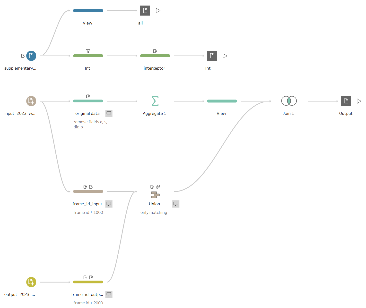
Flow 1: Contextual Data and Interceptor Identification
The first flow focused on isolating and enriching the supplementary data which provided critical contextual information about the game and play situation (e.g., down, yards_to_go, offense_formation, and the result, pass_result).
- Filtering: The data was initially filtered to include only rows where
pass_resultwas 'IN' (Intercepted pass). - Interceptor Extraction: A RegEx calculation was applied to the
play_descriptionfield to reliably extract the name of the interceptor. - Output: This flow produced a clean table containing the interceptor's name and all relevant play context fields.
Flow 2: Creating Continuous Movement Tracking
The second, more complex flow was designed to integrate the pre-throw tracking data (input_2023_w[01-18].csv) and the post-throw tracking data (output_2023_w[01-18].csv) into a single, continuous record of player movement.
- Frame ID Unification: A critical step was ensuring the
frame_ids were unique across the pre- and post-throw data. Since theframe_ids in both tables started at 1, they were not suitable for a direct union.- Input Frames: A constant value of 1000 was added to the input
frame_ids. - Output Frames: A constant value of 2000 was added to the output
frame_ids. This allowed the tables to be Union-ed into a single chronological sequence, distinguishing pre-throw movement (frames 1001, 1002, ...) from post-throw movement (frames 2001, 2002, ...).
- Input Frames: A constant value of 1000 was added to the input
- Data Reduction: The pre-throw data was streamlined by removing extraneous movement fields (
a,s,dir,o- acceleration, speed, direction, and orientation), as these were not required for the specific interception analysis. - Aggregation: The movement data was aggregated to ensure only distinct player/play information (e.g.,
player_name,player_position,ball_land_x,ball_land_y) was retained for each play, allowing this static information to be joined correctly to the multiple rows of movement data. - Final Join: The resulting movement data was then joined back to the contextual player and play information extracted from the input data to create the final analytical data set.
Read the next blog post for Day 5, containing the final build, outcome, and submission analysis.