Linear regression plot with Deneb

This blog is inspired by the following Workout Wednesday challenge (dataset in the link):

2023 Week 07 | Power BI: Non-linear Regression – Workout Wednesday (workout-wednesday.com)

I will be going through only the linear regression part, as I had an hour and a half to learn everything from opening the Deneb tool to creating a layered chart and using transforms (linear regression is a type of transform).

Here is my attempt:

And some useful documentation:

Examples gallery - https://vega.github.io/vega-lite/examples/

Linear regression - https://vega.github.io/vega-lite/examples/layer_point_line_regression.html

Colours and scales - https://vega.github.io/vega-lite/docs/scale.html#:~:text=By%20default%2C%20Vega-Lite%20assigns%20different%20default%20color%20schemes,color%20range%20%28the%20%22blues%22%20color%20scheme%20by%20default%29.

Scatter Plot

Deneb can generate a scatter plot automatically, from dragging fields into the "Visualizations" pane and then on the "Edit" view inside the tool.
But dragging a field into Series is mandatory at this stage and I only had two columns, so this was the result:

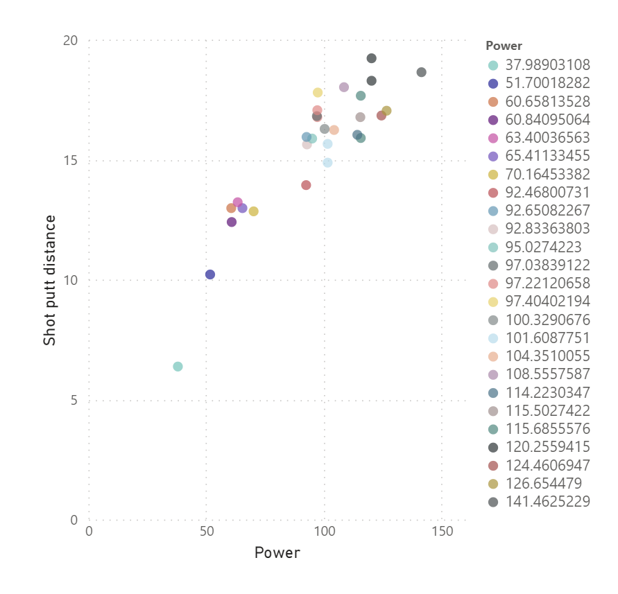
Not quite what we need, but a decent start.

Looking at the "Specification" tab, this is the code generated for the scatterplot:

{
    "data": { "name": "dataset" },
    "mark": { "type": "point" },
    "encoding": {
        "x": {
            "field": "Power",
            "type": "quantitative"
        },
        "y": {
            "field": "Shot putt distance",
            "type": "quantitative"
        },
        "color": {
            "field": "Power",
            "type": "nominal",
            "scale": {
                "scheme": "pbiColorNominal"
            }
        }
    }
}

We want to get rid of that "color" field, in particular the "nominal" type. For example, substituting "nominal" with "quantitative" changes the colour into a continuous palette. However, I did not to it at this stage. When layering multiple visualizations, adding colour works differently.

Layering Visualizations

Adding layers is just a matter of writing (or copy-pasting) the code for each new visualization in the "Specifications" view, as long as they are all wrapped into a "layer" function.

This is the final code for the viz:

{
  "data": {"name": "dataset"},
"layer": [
    {
      "mark": {
        "type": "point",
        "filled": true, 
        "color": "teal"
      },
      "encoding": {
        "x": {
          "field": "Power",
          "type": "quantitative"
        },
        "y": {
          "field": "Shot putt distance",
          "type": "quantitative"
          
        }
      }
      
    },
    {
      "mark": {
        "type": "line",
        "color": "grey"
      },
      "transform": [
        {
          "regression": "Shot putt distance",
          "on": "Power"
        }
      ],
      "encoding": {
        "x": {
          "field": "Power",
          "type": "quantitative"
        },
        "y": {
          "field": "Shot putt distance",
          "type": "quantitative"
        }
      }
    },
    {
      "transform": [
        {
          "regression": "Shot putt distance",
          "on": "Power",
          "params": true
        },
        {"calculate": "'R²: '+format(datum.rSquared, '.2f')", "as": "R2"}
      ],
      "mark": {
        "type": "text",
        "color": "black",
        "fontSize" : 16,
        "fontWeight" : "normal",
        "x": "width",
        "align": "right",
        "y": -5
      },
      "encoding": {
        "text": {"type": "nominal", "field": "R2"}
      }
    }
  ]
}

Author:

Maddalena Mariano

View Profile