


A Linear Regression aims to describe the correlation between one dependent variable and one or more independent variables.
In other words, this helps us understand if changes in one variable will also result in changes in another. This can be useful for predicting and estimating missing values in the sample (this process is known as interpolation).
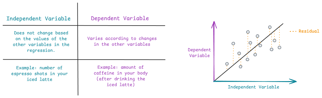
An ideal regression model would minimise the sum of the residuals - residuals are the difference between the line of best fit and the actual values. A value known as R2 (which ranges between 0 and 1) measures how much variability in the dependent variable explained by the line of best fit.
- A high R2 suggests that the model’s predictions are close to the actual value and therefore, a better fit for the data.
- A low R2 suggests that the model’s predictions explain little of the data’s variation and is a poor fit for the data.
Generally spaking, the higher the R2, the better your model.
How to Run a Linear Regression in Alteryx
Imagine you are a penguin researcher in Antarctica. You’ve been watching the penguins (from a safe distance!) for several months and have noticed that the larger penguins tend to have longer flippers. Since you dabble in statistics in your free time, you would like to find out if penguin body mass can predict flipper length.
This is something you can quickly find out in Alteryx.
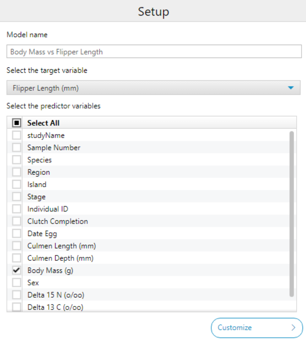
After loading in your penguin data and using the Select tool to ensure that your numerical fields are numeric (as regression models can only predict continuous values), you can now drag in the Linear Regression tool.
In the configuration pane, there are a number of things you can change:
- Model name - It’s always helpful to give your models a useful, unique name so it can helo you reference it in later workflow steps!
- Target variable - This is where you choose the outcome you want to predict (dependent variable).
- Predictor variable(s) - This is where you choose one or more fields to use as inputs for the model (independent variables).
- Other configuration options let you omit the model constant, apply record weights, enable regularisation, standardise predictors, use cross-validation with fold and seed settings, and choose between a simpler model or one with the lowest error. See more delta about the advanced customisation options here.
For our example, we can do the following to check if flipper length can be predicted by body mass:
You can then add a Browse tool onto each of the 3 output anchors to view the results of the regression model. There are 3 output anchors:
- O - This output delivers the regression model object which can be used in subsequent predictive tools for scoring or further analysis.
- R - This output generates a comprehensive report with model summary statistics, coefficients, residuals, R-squared values, and diagnostic plots to help interpret model performance and fit.
- I - This provides an interactive report that lets users explore diagnostics and summary information in an engaging format.
Interpreting a Linear Regression
If we click on the Browse tool for the R output, this is what we will see:
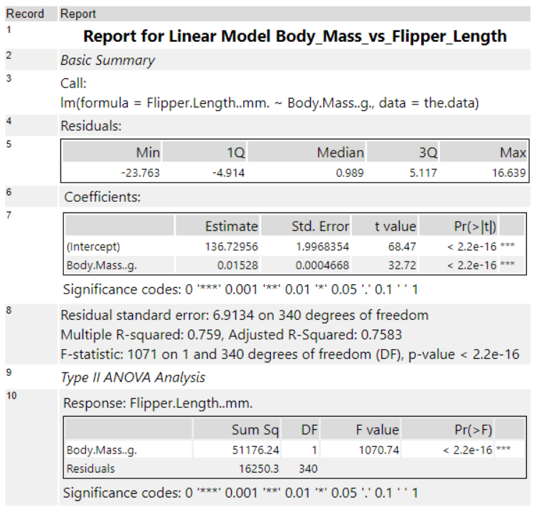
Although this view can be overwhelming, there is a lot of things we can learn about our data:
- The intercept (136.73) is the expected flipper length when body mass is zero. The coefficient for body mass (0.01528) shows that, for each additional gram of body mass, the flipper length increases by about 0.015 mm.
- Both coefficient p-values are very low (< 2.2e-16 ***) which means these predictors are highly statistically significant.
- The R2 of 0.759 suggests that about 76% of the variance in flipper length can be explained by body mass.
Overall, this means there’s a statistically significant and positive relationship between body mass and flipper length in the dataset. In other words, the regression model fits well and we can conclude that body mass is a reliable predictor for flipper length.
As you can see, running a linear regression in Alteryx is just as easy as that!