


Assigning rows of data to a group is typically done in Power BI using bins or lists. Once a row of data is assigned to a group, this remains static and it can no longer be updated using slicers or filters due to the order of operations. What if you do want these groups to be dynamic?
In this blog, part of the Explaining with series, I'll run through how to approach this as well as cover the basis of groups/bins and what it could be used for.
As per usual, the Power BI report is available on my Explaining with GitHub repository if you'd like to dive into it straight away.
How to group data and what can we use it for?
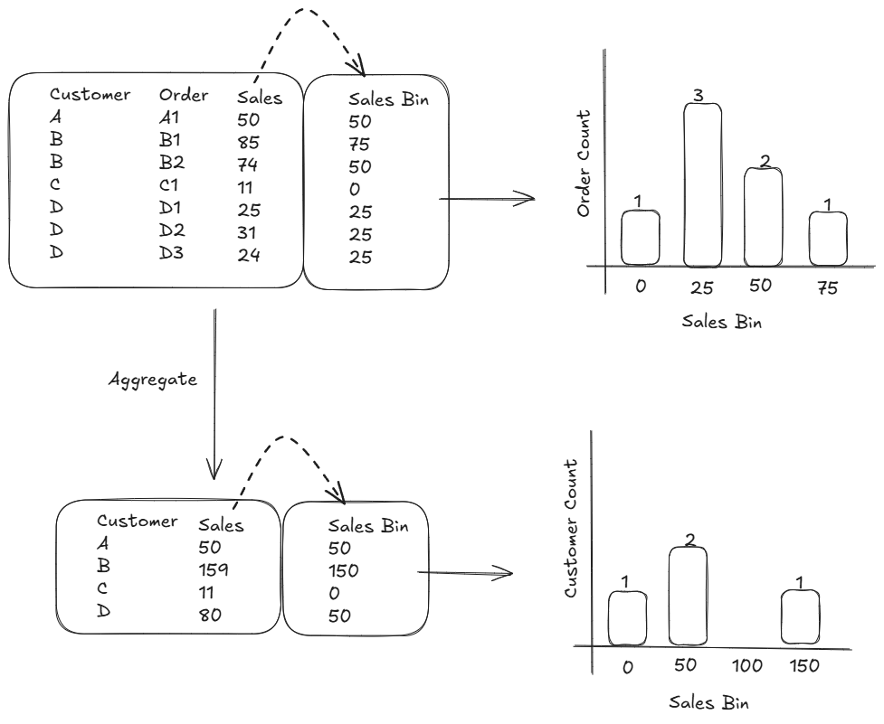
One of the main reasons we might want to group our data is to identify distributions in the data. For instance in the example below we can use our Sales data to group up orders into equal sized groups (bins) to build out distributions to identify a typical order size and to see what the 'value' of our customer base looks like.
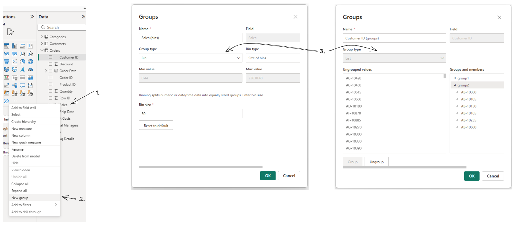
Both of these methods involve creating a new column in Power BI, we can use the equal sized bin feature (if the field is numeric) or create your own list (any field type) by right clicking on the column in the data pane > new group.
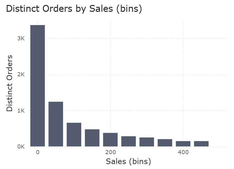
Once created, a new column appears in your data model and you can use it to visualise your distributions.
Why would you need dynamic bins?
If your bins can be created at a row level of your data, static bins are sufficient. However, there are plenty of use cases where we might want to re-calculate what bin a customer should be assigned to based on what slicers or filters are applied to your data.
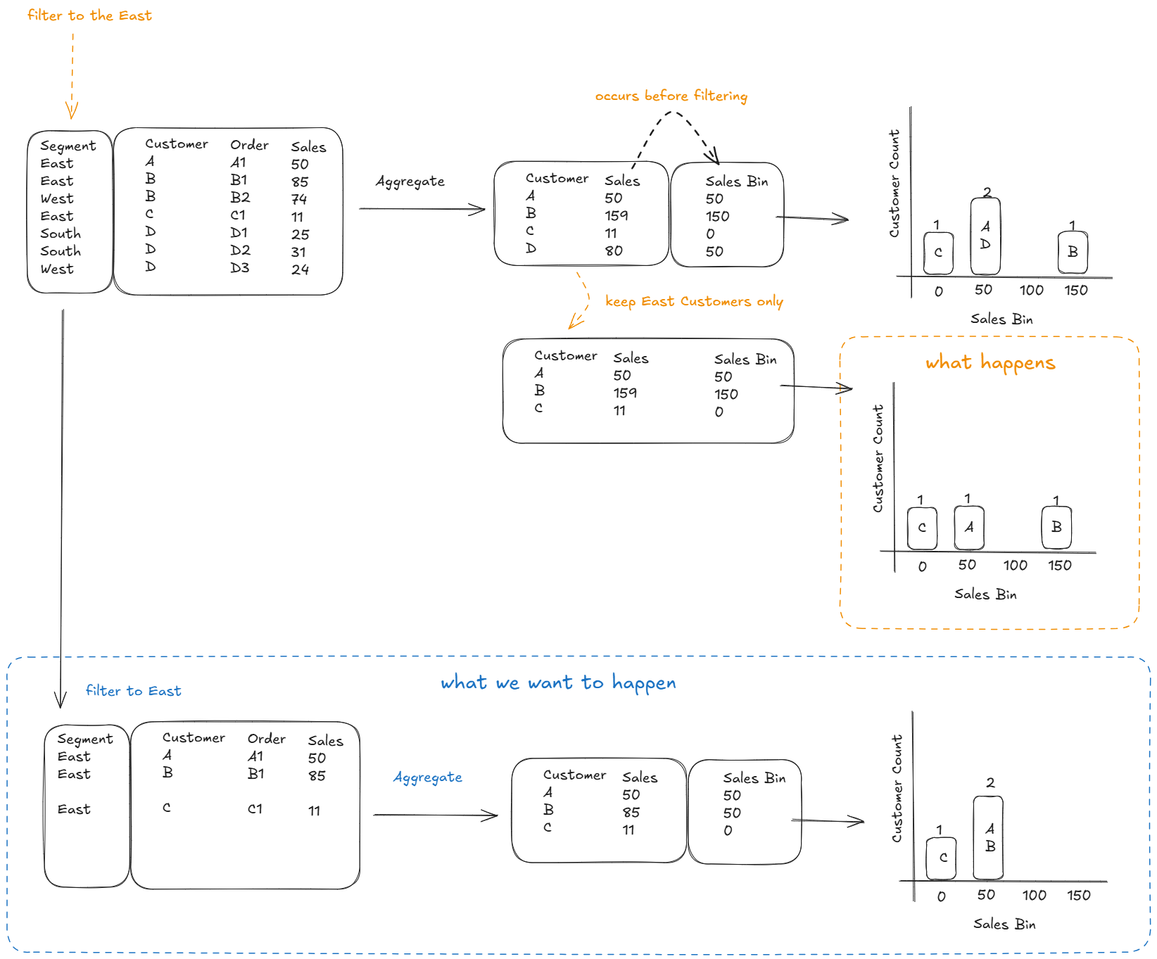
Let's take our previously used sample data where we want to see the distribution of customers based on how much they've spend with us in total.
We aggregate it to the customer level, creating a separate table (or use context transition using a column calculation but let's keep it simple for now), create our bins and visualise our distribution. We've grouped them into 3 bins, 0, 50 and 150.
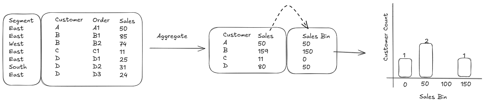
We now have an additional Report slicer we want to apply, where the end-user can filter to any Segment. Let's say, we select East.
Power BI filters the data to only rows in the East, the data model filters your customer sales table to only customers in the East and updates your visualisation. Customer D is left out, A, B and D remain but their assigned sales bins are not updated to reflect their Sales only in the East!
What we want to happen is that the groups are re-assigned after we filter our records to only the rows of data that contain East. So what's happening?
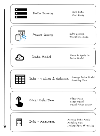
The order of operations in Power BI works through a series of steps, as outlined in the image below from top to bottom.
As the creation of groups falls under the DAX - Tables & Columns step, it means they will be materialized before the Slicer Selection. Regardless of what we try, we cannot get the 'grouping' step to happen after the slicer selection.
Thus our only option is to make use of DAX - Measures, that occur after Slicer Selection. I'll cover how to do this in the next section.
How to create Dynamic Groups
Now that we know why we can't use groups (basically Columns) when we want to dynamically group records, let's go over the solutions we have.
Before we create a measure that allow us to dynamically assign records to a group, we need to create the groups (as a table). This is required as we need a column to bring into a x or y axis that break up our visual.
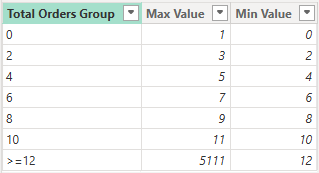
For this example, I'm using a data set where I'd like to group our Customers based on how many unique orders they have placed with us. The distribution we are going for is group sizes of 2 (0-1, 2-3, etc) until we reach 12 after which we class the rest as larger or equal to 12 (>=12)
You can hit the Enter data button in the Home Tab, but to keep things easy to edit I create a table using DAX.
Note that I have added a minimum and maximum column as well, these are required in the case where we have larger than 1 group sizes.
Total Order Group =
//You can hardcode the groups and numbers but this will make sure we never find values >= then the Max Value in the data set
//Keep this table disconnected from the data model
VAR _StaticTable =
DATATABLE(
    "Total Orders Group", STRING
    ,"Min Value",INTEGER //use Sort as the sort by column and inside your numeric checks
    ,"Max Value",INTEGER
    ,{
        {"0",0,1}
        ,{"2",2,3}
        ,{"4",4,5}
        ,{"6",6,7}
        ,{"8",8,9}
        ,{"10",10,11}
        }
)
VAR _maxOrders = [Distinct Orders]
VAR _LastRow =
{
    (">=12",12, _maxOrders)
}
RETURN
UNION(
    _StaticTable
    ,_LastRow
)
Table
This table will be unrelated to your data model and we will assign our customers to the right groups in our Measure.
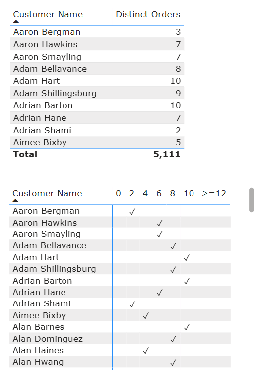
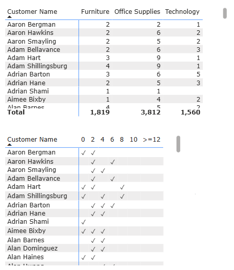
In the image below, we can see two tables. The first shows a list of our customer names and their Distinct Orders, DistinctCount( Orders[Order ID] ) Measure.
To test which group a customer belongs I've created the second table with a measure to populate the second table with ✓'s to test (do note that this calculation is not required for the final visuals, it is just to showcase the logic we will use later).
What Group am I part of? =
VAR _Min = SELECTEDVALUE('Total Order Group'[Min Value])
VAR _Max = SELECTEDVALUE('Total Order Group'[Max Value])
RETURN
MAXX(
    VALUES(Customers[Customer Name])
    ,IF(
        [Distinct Orders]>=_Min && [Distinct Orders]<=_Max
        ,"✓"
        )
)
Measure
We first capture the range of values from the groups in the variables and then compare it against the distinct orders of each customer to see if it's within the range. If yes, then ✓ else blank.
As we are comparing a measure (Distinct Orders), our assignment of groups will now respond to any filter or slicer, as measures are computed after the filters!
In order to now count how many (unique) customers are now part of each group we alter our measure above slightly by introducing the ALL() function to introduce the correct row level to our iterator function so we can count our customer names as they are not present inside our column chart (whereas in our table example we could use VALUES() as customer name is present).
Total Customers by Total Orders Group =
VAR _Min = SELECTEDVALUE('Total Order Group'[Min Value])
VAR _Max = SELECTEDVALUE('Total Order Group'[Max Value])
RETURN
SUMX(
    ALL(Customers[Customer Name]) //preferable to use ID columns as those should be unique, in this data set both are unique and names are used for example purposes //use ALLSELECTED if slicers are present that filter the column specified inside ALL
    ,IF(
        [Distinct Orders]>=_Min && [Distinct Orders]<=_Max
        ,1
        ,0
        )
)
Measure
See the Report in action below, or download it yourself from GitHub.
If you are after a solution for creating equal-sized bins with a dynamic range, I'd recommend watching the video below by @HowtoPowerBI
https://youtu.be/oa0sBSJBFe0?si=nYElrPcBZ2W1kUgd
How to incorporate Distinct Count into the Dynamic Grouping?
With the example above, we iterate over a unique list of customers and sum up the 1's created. This works well if that's the only column that determines the granularity for group assignment. So what if we introduce another column into the mix, e.g. a customer can be part of multiple groups depending on which category they bought products in.
Why would we do this? If we consider a business it could be that we consider customers unique depending on what section of the business they buy things from, or in a different scenario, which part of our GP service did they go?
When we eventually count how many patients have come to us they can be part of group 0-1 if they came once for a blood test and group 4-5 if they saw the nurse four times. It's a niche use case, but nevertheless something our clients have requested before.
In this example, I used [Category] together with [Customer Name], who both come from separate tables in our data model, linked through the orders table.
We have to slightly alter the DAX for both measures compared to our previous example.
What Group am I part of? (Multiple Groups) =
VAR _Min = SELECTEDVALUE('Total Order Group'[Min Value])
VAR _Max = SELECTEDVALUE('Total Order Group'[Max Value])
VAR _Table =
SUMMARIZE(
    Orders,
    Categories[Category]
    ,Customers[Customer Name]
)
RETURN
MAXX(
    _Table
    ,IF(
        [Distinct Orders]>=_Min && [Distinct Orders]<=_Max
        ,"✓"
        )
)
Measure
Note that I use SUMMARIZE() to achieve the desired output, due to the fact both columns are from separate tables. Creating the unique list of customer names and categories to iterative over to assign customers to their groups.
The next measure had to be expanded on in order to achieve a distinct count of a customer name when it appears more than once in a assigned group. Using the same SUMX() with 1's and 0's would count a customer name twice if they'd appear twice in the same group.
As there is no DISTINCTCOUNTX() we use a COUNTROWS() over the DISTINCT() function of a table to achieve the same. The groups are pre-calculated in the _GroupTable variable and is used to filter our distinct count to the correct groups.
Distinct Customers by Total Order Group (Multiple Groups) =
VAR _Min = SELECTEDVALUE('Total Order Group'[Min Value])
VAR _Max = SELECTEDVALUE('Total Order Group'[Max Value])
VAR _GroupTable =
//your data model allows, use ADDCOLLUMNS( ALLSELECTED( ) ), in this data model Category and Customers live in seperate tables
SUMMARIZE(
    Orders,
    Categories[Category]
    ,Customers[Customer Name]
    ,"Distinct Orders", [Distinct Orders]
    ,"Groups", IF(
        [Distinct Orders]>=_Min && [Distinct Orders]<=_Max
        ,_Max
    )
)
VAR _DistinctCustomersPerGroup =
CALCULATE(
    COUNTROWS(
        DISTINCT(
            ALLSELECTED(Customers[Customer Name])
        )
    )
    ,FILTER(
        _GroupTable
        ,[Groups]=_Max
    )
)
RETURN
_DistinctCustomersPerGroup
Measure
And there we are, an introduction to dynamic grouping in Power BI using DAX.