For those of you who don’t know what Preppin’ Data is about, it’s an initiative of Coach Carl and my fellow cohortian Jon to popularise Tableau Prep in a weekly series of challenges. It works in a similar way to Alteryx Community Weekly Challenges, where you’re presented with input data and the expected outcome, and the task is to figure out the flow that gets you from point A to point B. For more info, check their blog.

It’s been almost a whole week since Week 2 problem was published and I thought (or rather Carl thought…) I give you a short summary of the problem and solution 🙂

Problem

This is the preview of the dataset (in Excel, sorry):

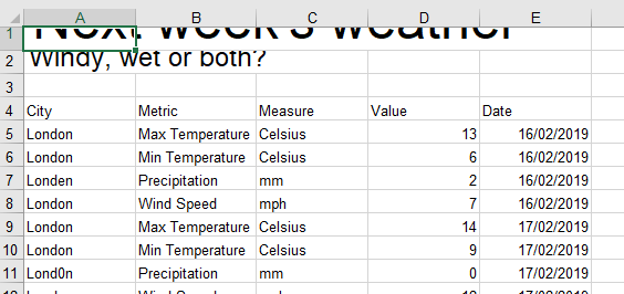
As you can see, we have some fancy headers at the top of the spreadsheet and there’s some extra space between data for London and Edinburgh. Another thing to notice (not so obvious from the snippets above) is that the values for City field have some interesting typos in them. The expected output also had separate fields for all Metric and Measure combinations.

Solution

Wildcard Input

First of all, you need to upload your data. I know there are a few things to do it but I used the data interpreter (my new friend), which quite accurately splits the whole sheet into two tables, and then used the wildcard option:

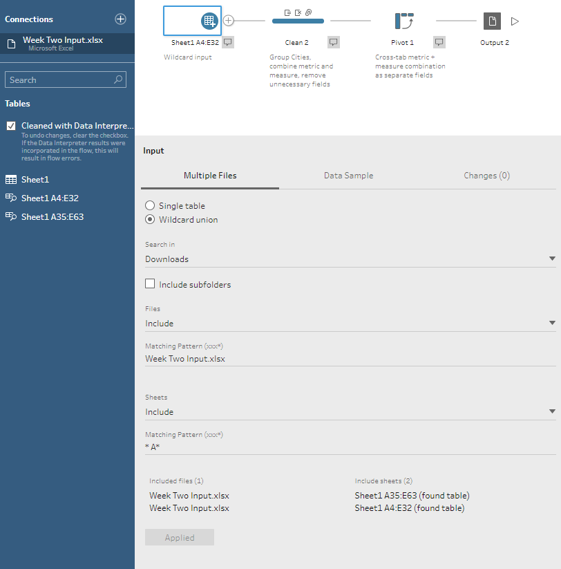
For a matching pattern in sheet names, I put ‘* A*’ which takes anything that has ‘ A’ in its name. ‘*’ is the wildcard which takes anything. This way we have both tables loaded as one. Noice.

Group and Replace

Moving on, we need to sort out our cities. Once you add the clean step, right-click on the City field -> Group and Replace -> Spelling. This will magically pick the values with similar spelling and group them together assigning the most common value. You can overwrite the automatic grouping by clicking on the group:

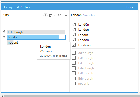
In the screenshot above, you can see one value that should be in London group, just check its box on the right-hand side. To rename the whole group, either click on three dots in the window on the left or double-click on the group on the left. Sweet.

Combine Metric and Measure

This is easy, just requires one calculated field (I called it ‘Metric – measure’, the name doesn’t make much of a difference here):

[Metric] + ' - ' + [Measure]

It just concatenates the texts in the Metric and Measure fields together.

Now we can get rid of unnecessary fields. For me these would be: Metric, Measure, Table Names, File Paths. The last two are automatically generated when using a wildcard input.

Pivot Rows to Columns

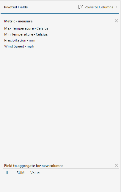
In Alteryx, this is a separate tool. In Prep, this is an option within Pivot tool. Columns to Rows is the default option. To change it, click on the caret next ‘Columns to Rows’ in the Pivoted Fields pane. Whoa… Then I dragged my calculated field (Metric – measure) on ‘Fields that will pivot rows to columns’ or the upper part of the Pivot Fields pane and Value field on ‘Field to aggregate for new columns’. It will automatically set the aggregation method to sum which is fine as there should only be one value per specific date.

Output

Make sure to output your data in a format of your choice. It can be .csv .hyper or .tde. That’s it!

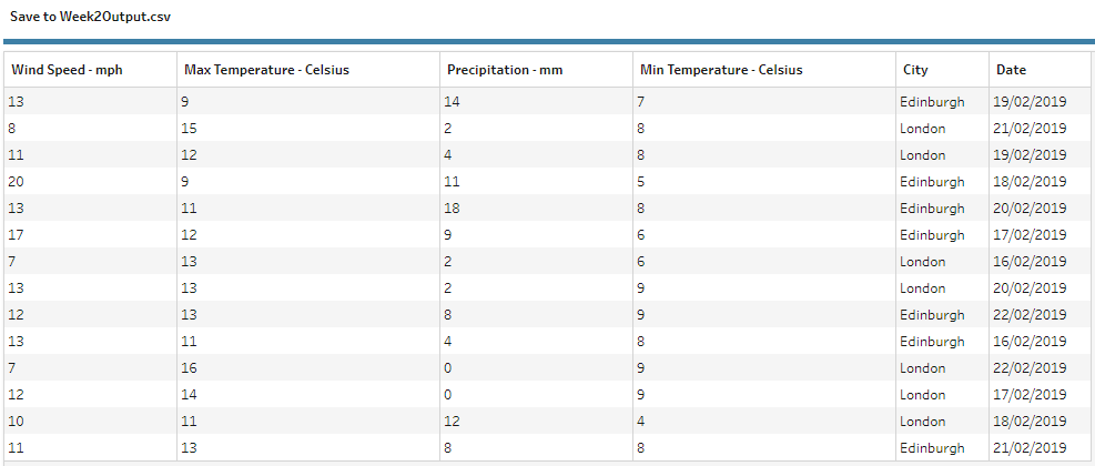
That’s much easier to process than the original data set…

If you haven’t already, have a look at the Preppin’ Data blog and start Preppin’!