In this blog, I’ll be working through the Preppin’ Data challenge called “Targets for DSB”. Check it out here! Like my other recent articles, I will be using SQL for this challenge.

Since this challenge is a continuation of the previous two weeks, a lot of the input data and data cleaning steps will be familiar to those of you who have already completed the aforementioned challenges.

This challenge is a real fun one because it requires changing the shape of a table that then will be joined to another table. Once that join takes place, a constructed field is made based on fields from both tables. Let’s dive in!

The input tables are pictured below.

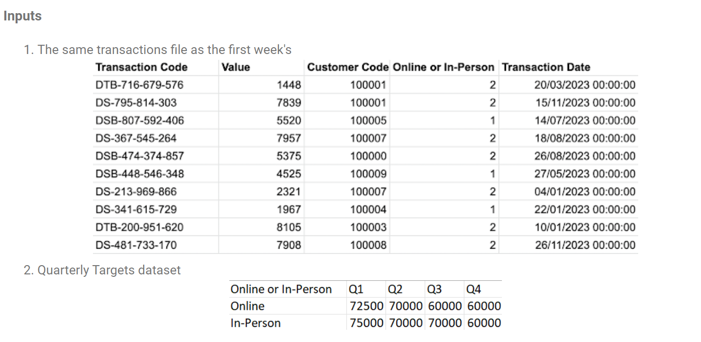
To complete this challenge, I opted to create two CTEs (trans and targs) and then join them together. Something to note from the above picture is how the shape of the two tables are totally different. This will be a major aspect of completing this challenge.

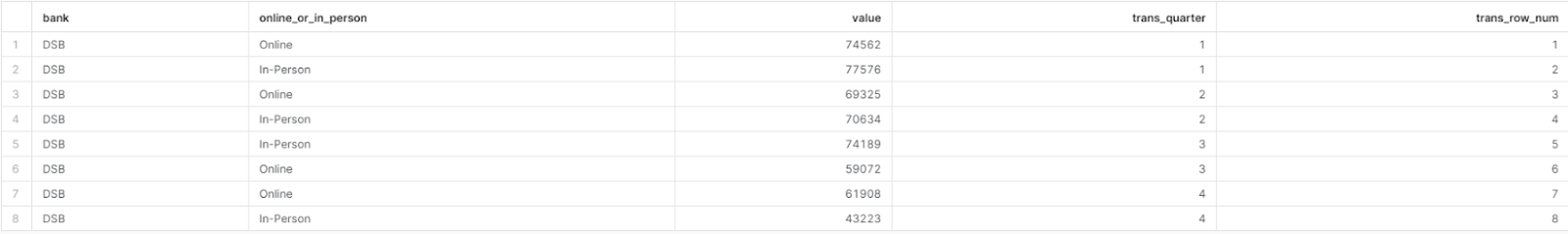
Let’s take a look at how the trans and targs CTEs were created and their outputs. The first query snippet and output relates to the trans CTE.

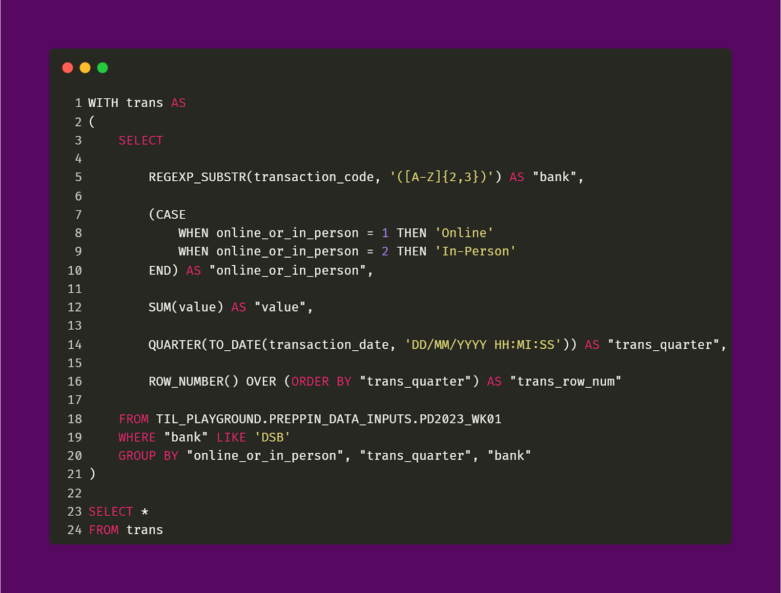
As I mentioned earlier, a lot of the cleaning for this CTE is familiar to us. For one, we need to create a Bank field from the Transaction Code field from the first input table. This can be done by using the REGEXP_SUBSTR function. What I’m doing here is to extract the string of characters that matches with the RegEx pattern of ([A-Z]{2,3}). This looks for any string of characters, that has a length of 2 or 3, that begins with any uppercase letter. This lets me avoid having to capture the hyphen symbol. So, I only get strings like "DS" and "DSB". However, as I mentioned in previous articles about being careful with using RegEx, I could also capture unneeded strings like "UP" or "PIE" if such substrings existed in the Transaction Code field.

Another familiar cleaning step is to modify the Online or In-Person field. A simple CASE statement can be used to associate the original value of 1 or 2 to their intended values of “Online” and "In-Person", respectively.

The last familiar cleaning step to do is to convert the original Transaction Date field to be a proper date field which conveys quarters in a year.

While it may not strictly be necessary in order to solve this challenge in general, I decided to create an additional field called Row Number for both CTEs. This simply numbers each of the rows of both CTEs in order. I did this because I will use this newly added Row Number field as an additional join condition. I will speak more about this later on as the concept of joining is very important for this challenge.

To be clear, the challenge requires two join conditions, one of which involves the Quarter field. The other join condition has to also be something that uniquely identifies each row in each table, such as the Online or In-Person field. However, for my approach to this challenge, I didn't use the Online or In-Person field from my CTEs.

Now, for the targs CTE. Its query snippet and output are shown below.

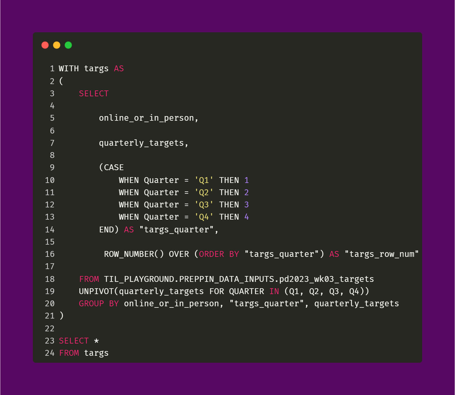
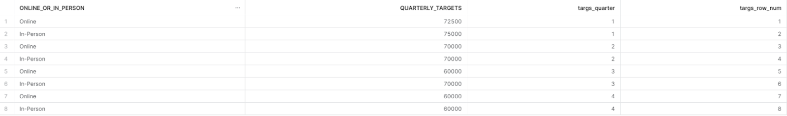
The query and results for the Online or In-Person and Row Number fields for the targs CTE is the same as in the trans CTE.

The Quarter field is created by using a simple CASE statement that assigns a quarter value (1 to 4) based on the original Q1 to Q4 fields from the second input table. An alternative to the CASE statement would be to use the SPLIT function or REPLACE function to remove the "Q" from the Q1 to Q4 fields.

The Quarterly Targets field is created by using the UNPIVOT function. This function converts field headers into row values. I think of it as "rotating" the table so that instead of having many fields (being wide), the table has many rows (being tall). This article does a great job at visualizing the difference between the PIVOT and UNPIVOT functions. Ultimately, through the UNPIVOT function, we are maintaining the pair between the Q1 to Q4 fields and their respective values. So, for example, Q1 has the values of 72500 and 70000 (based on whether or not a transaction is "Online" or "In-Person"). These values do not get changed (like they would be if the PIVOT function were to be used).

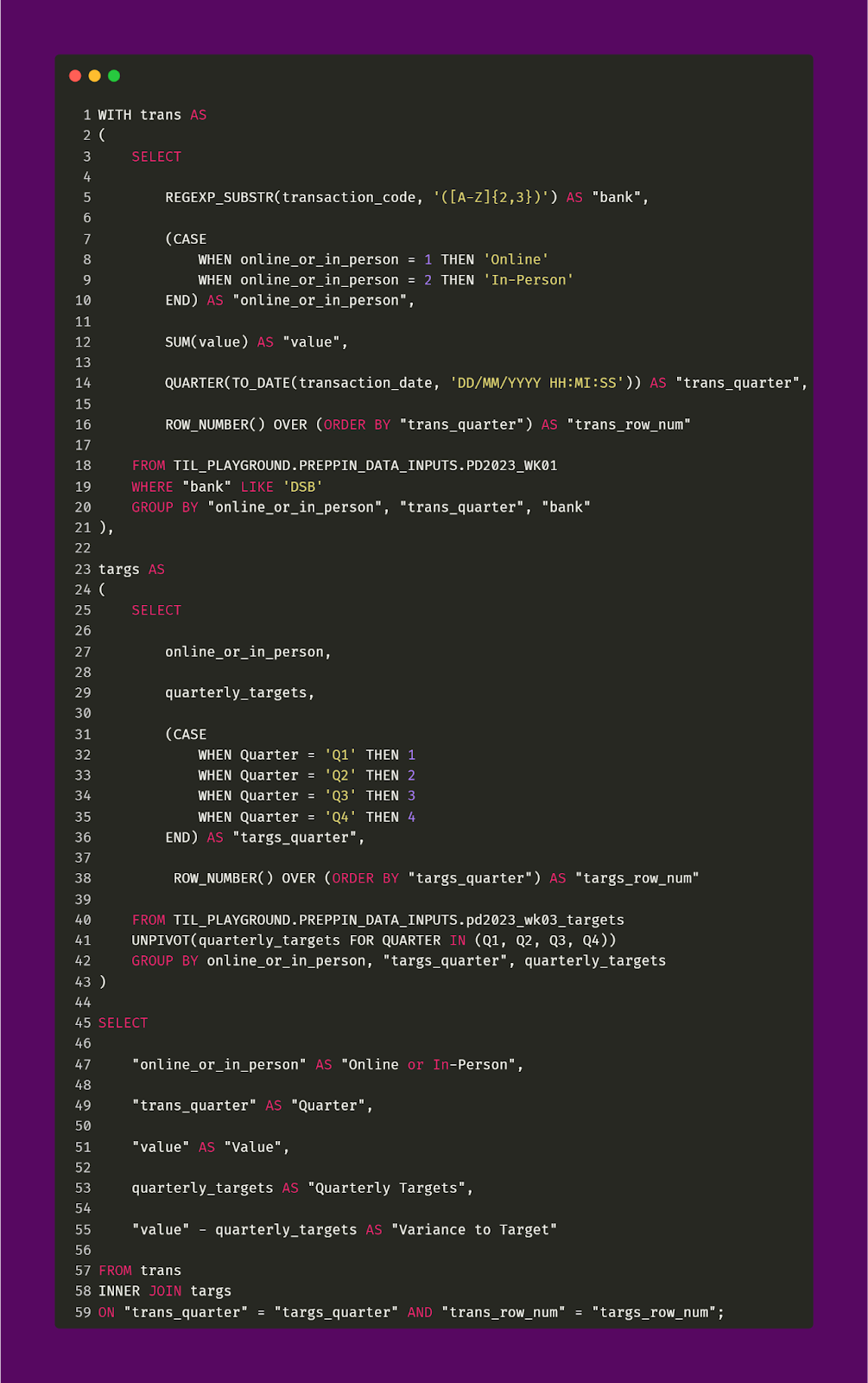
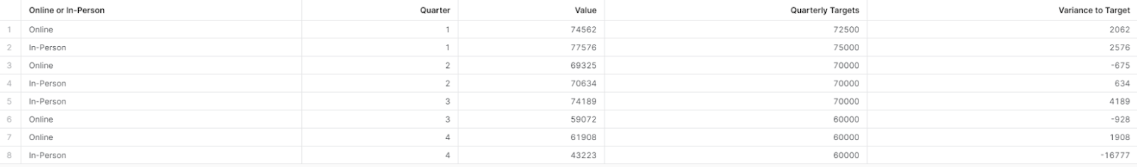
With all of that said, let’s consolidate these two CTEs. The query snippet and output are shown below.

This was a solid challenge demonstrating the importance of being careful about how to join tables together. If we get that wrong, we can end up introducing duplicate rows (or other data errors) into our result table. This could prove disastrous because it means that KPIs could be calculated incorrectly, for example. More than that, we could be working with needlessly large tables that may introduce performance problems and additional expenses with respect to data storage, data querying, migration of data and products that tie into said data, dashboard development and other business processes that would utilize the erroneously large table.

To illustrate what I mean about the dangers of improper joining, let’s look at a supplemental output that represents the query above when the second join condition (Row Number fields) is removed.

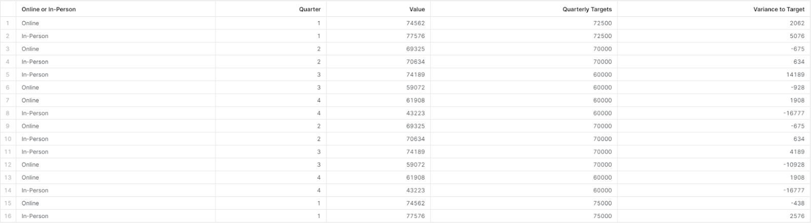
As you can see, if we only join the CTEs on the first join condition (Quarter fields) we get a result table that is 16 rows instead of 8 rows. With this, we have introduced duplicate rows and inaccurate data.