


Predictive models, or a variation of machine learning, can be very powerful tools in data analytics as they can provide calculated and weighted answers to questions which would be otherwise estimated. In reality these tools are actually well thought-over estimates to a question that the machine has seen the answer to under many different parameter values. The machine sees how the answers have previously depended on the parameters involved and gives its estimate as to what the answer is likely to be for this new set of parameter values. Due to how the data is arranged some models may be better than others, so before committing to a certain model to predict your data it can be a good idea to compare a few.
Firstly, you will need the predictive tools downloaded. Alteryx will come with 3 already in the toolbar but don’t be fooled, these aren’t the only predictive weapons Alteryx possesses! If you do not have the predictive tool already installed then download the package from here making sure to select the correct version of Alteryx you are using.
In this example we will be using data on different stores, including information on customers, the location and amount of different cars sold, as well as the sum of the sales for each store. In this example with information about customers, location and amount of cars sold will be our predictors and the sum of sales will be our target. This is to say that the machine will see how the predictors affect the target, so how the different types of customer, location and cars sold affects the sum of sales for that store. Before starting make sure all the continuous predictors you wish to use are formatted to be a number.
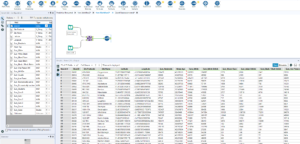
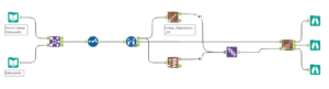
As we are testing multiple models we need to take a sample of the data for the models to learn from and a sample of the data for the models to compare their answers against. These are called the ‘estimation sample’ and ‘validation sample’. To create these samples we need to use to ‘Create Samples’ tool in Preparation. The Create Samples tool allows you to chose the percentage of the data that is used for the estimation, the percentage of the data that is used for the validation and how much of the data is not used. With reasonably sized data sets a good ratio is around 80% for the estimation and 20% for the validation, however this can vary. For very large data sets the model will take a very long time to run and might be at risk of overfitting, so it can be useful to leave some of the information out. For this example the ratio of 80% to 20% will be used.
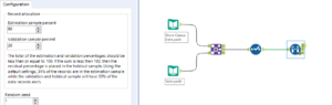
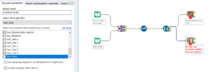
The estimation data will be outputted from the ‘E’ tab at the top, the validation data will be outputted from the ‘V’ tab in the middle and the unused, or ‘hold out’ data, will be outputted from the ‘H’ tab. So from the ‘E’ tab the different models need to be set up. Here we will compare how Linear Regression compares against the Boosted Model. Set these up by selecting Sum_Sales as the target field and all the predictors as the predictor fields (make sure not to include the target field within the predictor fields!). Also if using Linear Regression the version of the model will have to be changed to 1.0 which can be done by right-clicking the tool and going to ‘Choose Tool Version’.
Adding a browse tool to the ‘R’ tab on the models will show a report of the model, but it is the ‘O’ tab which will output the data to be used. Next we need to union the results of the two models together. To do this we take the ‘O’ output from both the model tabs to a Union tool and leave the Union to auto config by name.
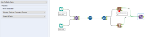
The next tool to be used may also need to be downloaded. The ‘Model Comparison’ tool can be downloaded here and then used in our comparison. The Model Comparison tool has two inputs, the ‘D’ input, to which data is inputted, and the ‘M’ input, to which the model data is inputted. Our data will be the validation data and the model will come from the union of the two models. Adding a browse tool to all three of the outputs (Ctrl+Shift+B for the keyboard shortcut) will show comparisons between the two models. The ‘E’ output gives the model information, the ‘P’ output gives actual data and the ‘R’ output gives the report.
The ‘E’ output tab is the one of interest here. Using the browse tool to see the results we can see 6 new fields. The ‘Model’ field is the model name being compared, the ‘Correlation’ field is how strongly the actual values correlate to the estimation line, and the ‘RMSE’ field is the sum of all the predictive errors from the actual value. The other three, provide more information (if you know how to use this information then please comment below) however we only need the first three to make a judgement. Firstly we want the ‘Correlation’ field to be as close to 1 as possible, as the closer the to 1 the value is the closer the estimation line is to being perfectly hitting all values. Secondly we want the ‘RMSE’ field to be as small as possible. As ‘RMSE’ is the distance between the estimated values and the real values the lower the better.
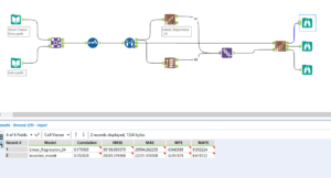
Here we can see that the linear model has a correlation of 0.17 and the boosted model has a correlation of 0.70. So the boosted model definitely wins here. Also the boosted model has a smaller RMSE score, so it is clear here that the boosted model trumps the linear model for this data set.
Other types of models can be compared in the same way and as many models as you want too. Changing the amount of data that is being learnt from and is being validated against will change how close the approximations are, so a balance needs to be made. A lot of the time one of the models will stand out as better amongst the rest but sometimes they might have to be looked into a little more.